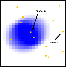
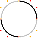
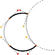
Sextant: A Unified Node and Event Localization Framework Using Non-Convex Constraints

Saikat Guha, Rohan Narayan Murty, Emin Gün Sirer
Dept. of Computer Science
Cornell University
Ithaca, NY 14853
{saikat,rnm5,egs}@cs.cornell.edu

Abstract:
Determining node and event locations is a canonical task for many wireless network applications. Yet dedicated infrastructure for determining position information is expensive, energy-consuming, and simply unavailable in many deployment scenarios. This paper presents an accurate, cheap and scalable framework, called Sextant, for determining node position and event location in sensor networks. Sextant operates by setting up and solving a system of geographic constraints based on connectivity information from the underlying communication network. Sextant achieves high accuracy by enabling non-convex constraints to be used to refine position estimates. It represents position estimates as potentially non-contiguous collections of points. This general representation enables Sextant to use _negative information_, that is, information on where a node or event is not located, to refine location estimates. Sextant unifies both node and event detection within the same general framework. It can provide high precision without dedicated localization hardware by aggressively extracting constraints from the link layer, representing areas precisely with Bézier-enclosed polygons and probability distributions, and using event detection to refine node position estimates. A compact representation and a fully distributed implementation make the framework practical for resource-limited devices. The framework has been implemented, deployed and tested on laptops, PDAs and Mica-2 motes. Physical experiments show that a large number (98%) of the nodes in a network can determine their positions based on a small number (30%) of landmark nodes and that a large number (90%) of events can be located with low median error.

1 Introduction

Many critical applications for wireless networks require determining the physical location of nodes and events in the network. For instance, a canonical problem in sensor networks is to determine the location of an event, such as a chemical spill. Geographic routing protocols rely on node location in order to forward packets with low overhead. Similarly, context-aware applications need to determine the locations of network participants in order to customize content for users depending on their location. These, and many other location-sensitive applications [1, 2, 3, 4, 5], require determining position information with high accuracy and low cost.

In this paper, we present a distributed location discovery framework, called Sextant, that extracts geographic constraints from already-present wireless radios and uses these constraints to infer node and event location with high accuracy. Sextant operates by setting up a system of relative geographic constraints among the network participants based on network connectivity and solving this system in a distributed and efficient manner with the aid of absolute position information provided by a small number of landmarks. A landmark is a node whose absolute position is known; Sextant landmarks can be cheap static nodes whose positions are fixed, or they may be mobile nodes equipped with dedicated hardware, such as GPS.

Sextant provides a unified framework that can be used to determine both node and event location. Sextant nodes equipped with sensors can extract and combine constraints about sensed events to cooperatively determine the geographic location of events. This location is represented as a probability distribution over the sensed area, which enables application-specific processing to be applied in determining the event location. Sextant relies solely on simple, cheap hardware for localization; a wireless radio and a binary event sensor suffice for both node and event localization, and costly hardware and protocols for time synchronization are not needed. Folding both event and node localization into the same framework enables sensed events to be used to improve the fidelity of node location estimates.

There has been much previous work on node localization and event detection [6, 7, 8, 9, 10, 11, 12, 13, 14, 15, 16] , including foundational work on theoretical lower bounds [17, 18]. Sextant differentiates itself from this body of work in several ways. First, it does not assume uniform transmission radii (i.e. a unit disk graph) or symmetric connectivity; instead it extracts geographic constraints from the link layer based on a novel, realistic constraint extraction model that accommodates the large percentage of unidirectional links and non-uniform coverage areas encountered in practice. These constraints lead to non-convex solutions, which are typically much more accurate, though more complex, than schemes limited to convex embeddings. They also naturally support event detection with heterogeneous sensors, where wide-area sensors may determine an event to have occurred in region R, while more specific sensors might preclude the presence of that event in smaller sub-regions S, S ⊂ R, giving rise to non-convex event regions. Second, Sextant explicitly represents node locations using Bézier curves, and uses probability distributions to track potential event locations. In contrast with some previous work that represented location estimates as points, representing areas and probability distribution over areas explicitly vastly improves localization accuracy, and Bézier curves greatly reduce the amount of space required to represent complex, non-convex areas. We show how to extend and combine areas made up of piecewise Bézier curves, and the scheme is simple to generalize to 3D with Bézier surfaces. Third, Sextant propagates constraints throughout the network, and can merge them effectively even in the presence of approximate information. In contrast with some past work that required landmark nodes in the one-hop neighborhood in order to perform node localization, Sextant can derive accurate constraints even from nodes whose position is not precisely known, and use these estimates to refine the position estimates of other nodes. Finally, we have deployed and tested our scheme on physical testbeds consisting of laptops and handheld HP Jornadas equipped with 802.11b cards, as well as 50 Mica-2 motes. The algorithm is practical enough to be deployed on motes, and robust enough to handle non-uniform behavior encountered in real networks.

Sextant aggressively extracts positive and negative information from the link layer and converts it into geographical constraints. By positive information, we mean a constraint that restricts a node's or event's location to a region of finite size. For instance, much past work is based on estimating a node's position by examining its hop count to landmark nodes [19, 9] or triangulation to landmark nodes in the one-hop vicinity [20]. Sextant additionally takes advantage of negative information; that is, constraints that preclude a node or event from appearing in a certain region. For instance, a node that does not receive transmissions from another node may determine that it is outside the transmission range of the sender. We show later that the use of such negative information greatly increases the fidelity of location estimates for both nodes and events.

We show how to use Bézier curves to explicitly represent the set of all points at which a node can be located. Since this set may consist of disjoint polygons, explicitly representing it as a set avoids estimation errors. Bézier curves are resilient to small errors in the location of control points [21], and in addition, can be represented very efficiently, reducing packet size. Sextant can pass this set to location-aware applications that can handle sets of positions, or perform a final mapping to a point in order to support legacy applications without introducing errors into the system.

Sextant disseminates constraints transitively throughout the network, creating an interdependent web. Transitively propagating location information enables nodes that are not within the immediate vicinity of landmarks to determine their location. It also enables nodes to extract negative information by discovering the presence and estimated location of other nodes in the network. Transitively combining position estimates enables information from sparsely distributed landmarks to be coalesced together to reduce positioning error.

Overall, this paper makes three contributions. First, it describes a unified localization framework for node and event localization. The framework achieves high accuracy by using non-convex regions to represent node and event locations, taking advantage of negative as well as positive constraints, and disseminating constraints transitively throughout the network. Internally, constraints are represented precisely and in compact form as collections of polygons enclosed in Bézier curves, resulting in an accurate and efficient implementation. Second, this paper proposes a novel and realistic constraint extraction model, and a distributed constraint solution algorithm. The constraint extraction model enables Sextant to aggressively extract constraints from existing hardware such as wireless radios and sensors. The distributed algorithm for solving the resulting constraint system is efficient and scalable. This algorithm enables nodes without any dedicated positioning hardware to determine their own position and the location of events with high accuracy based on a small number of landmarks. Finally, this paper reports results from an actual physical deployment as well as simulations to show that the approach is both effective and practical. We have implemented the location discovery protocol described in this paper and tested it on MICA-2 motes [22], laptops and StrongArm-based PDAs equipped with 802.11b cards. The physical experiment validates the simulations, and shows that Sextant is effective at accurate location discovery.

The rest of the paper is structured as follows. The next section discusses related work and expands on Sextant's contributions. In sections 3 through 6, we discuss the basic operation of Sextant, including its area representation, its extraction of constraints from wireless radios and sensors, and its distributed solution techniques for node and event localization. Section 7 describes how the interaction between node and event localization can be used to refine position estimates. Section 8 describes the network protocol used to obtain and combine position estimates. Section 9 outlines the structure and complexity of the Sextant implementation. Section 10 provides results from our simulations and physical experiments and Section 11 concludes the paper.

2 Related Work

There has been extensive past work on node localization as well as event tracking in sensor networks (see [23] for a survey). These systems differ in the way they obtain range measurements, propagate location estimates transitively, utilize positive versus negative information, and represent potential node locations.

Range measurements can be obtained through simple connectivity, signal strength, time of arrival, time difference of arrival or angle of arrival measurements. Recent work has examined heuristics for performing range measurements via hop counts [13]. Sextant is agnostic to the choice of range measurements, and assumes the simplest form of range measurements based on connectivity, which is available from any wireless radio. Dedicated hardware for localization is costly and unavailable under many scenarios.

A common approach to estimating node positions is direct measurement or triangulation against landmarks in the immediate one-hop vicinity. Active Badge [24] relies on the closest infrared receiver to locate specialized beacons carried by tracked assets. RADAR [19] relies on a centralized database of signal fingerprints from landmarks obtained at all locations and orientations to localize a node. Lorincz and Welsh [14] propose a similar RF fingerprint-based node localization technique that relies on strength signatures and a distributed database. Cricket [25] relies on time difference of arrival between radio and ultrasound signals to measure distances to dedicated beacons. VORBA [26] uses angle of arrival measurements from 802.11 basestations to determine node positions. In GPS-Less [27], a node that can receive transmissions from landmarks L1, L2 and L3 estimates that it is at the centroid of the landmarks. Since these approaches do not disseminate position estimates beyond the first hop, they do not support nodes that are outside the range of landmarks.

Other work enables location estimates to be extended transitively through the network to nodes that are not within the immediate vicinity of landmarks. APS [9] relies on signal strength or hop counts for triangulation and estimates node positions starting with the one-hop neighborhood of landmark nodes and working transitively. A variant of APS [8] relies on angle of arrival measurements to perform triangulation and transitively determine position and orientation for nodes. GPS-Free [28] relies on time of arrival measurements to estimate the range between pairs of nodes, constructs local coordinate systems at each node, and reconciles them into a single, absolute coordinate space. Time of arrival and angle of arrival measurements are typically not practical since they require costly clock synchronization hardware and receiver arrays, respectively. Robust Positioning [20] is a two-phase approach where a system of loose constraints, built initially by range estimates, are iteratively refined to improve estimated locations. Robust positioning is agnostic to the choice of range measurements, but iterative refinement may never converge, even for static networks. Convex position estimation [29] solves a set of convex geographic constraints in a centralized server to localize nodes. Finally, N-hop Multilateration [30] combines robust positioning and convex position estimation to formulate a least-squares problem to refine initial position estimates. These approaches differ fundamentally from Sextant in that they use only positive information and work only with convex constraints.

The system proposed by Galstyan et al. [10] is similar in spirit to our approach in that it takes advantage of negative information. Information on where a node or event cannot be located can significantly improve the fidelity of location estimates. The system proposed by Galstyan et al., however, does not support non-convex position estimates. Non-convex areas, that is, areas with a missing subregion, arise naturally from the use of negative information, though representing them accurately is a challenge. This scheme simply uses the largest convex subregion instead, and requires that each node be in range of at least one landmark.

A significant difference among node localization techniques is the way they represent estimated locations. Most previous work computes a position estimate consisting of a single point for each node. Such an estimate might be wildly misleading; for instance, there might be sufficient information to indicate that a node is at the upper-right, upper-left, lower-right or lower-left parts of the field. A single point estimate may place the node at the center of the field. Galstyan et al.'s approach represents an estimated area as a rectangle, while Sextant represents areas explicitly as a collection of polygons enclosed by Bézier curves.

In addition to node localization, there has been much work on event tracking and localization. In collaborative Signal and Information Processing [31], the path of moving objects are tracked in a field of location aware sensors. The event location is derived from the magnitude of the sensor reading, given the attenuation model for the event. Acoustic Ranging in Sensor Networks [32] locates sound sources to a point location by triangulating against a set of landmark sensors that detect the event. Brooks et al. [16] propose a distributed target tracking system using a publish-subscribe model. Their work assumes that each sensor is equipped with a GPS for localization and instead focuses on the use of pheromone routing, in-network filtering and object tracking. Savvides et al. [12] propose an iterative event localization scheme based on measurements of signal strength. Energy-Efficient Surveillance System [33] also detects events in a location aware sensor field and routes back results along a gradient set up by the controller. This approach is centralized and relies on time synchronization. In the Countersniper system [11], event localization is performed using accurate time of arrival estimates and node localization is performed using acoustic ranging. This approach relies on tight time synchronization between sensor nodes and requires each sensor to be in the range of at least four other sensors in order to accurately localize the event, thus restricting the possibilities of dynamic configurations of sensor deployments. In contrast, Sextant can determine the location of events based on their signatures, without time synchronization.

The most significant difference between our approach and previous work is that Sextant is practical. It derives this property from its constraint model, which takes advantage of negative constraints, and its solution technique, which is distributed, transitive, and most importantly, capable of handling non-convex areas. Introduction of non-convex areas qualitatively changes the approach from previous efforts, such as [6], that are limited to convex regions. Some recent work has examined how to derive node locations without the benefit of any landmarks [7, 18]. Theoretical analyses have established estimation lower bounds for unit disk graph embeddings without landmarks [17]. The problem that Sextant tackles is more difficult than a unit disk graph embedding since it admits non-convex areas, though the use of landmarks simplifies the problem space. As a result, we have deployed and tested Sextant in practice, and later show that it achieves high accuracy in a real world setting.

3 Representing Regions and Positions

(a)

(b)

(c)

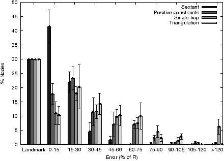
Figure 1: Use of Bézier curves to represent the area (a) enclosed by a circle, (b) common to two circles, (c) inside one circle but outside another. Control points are represented by filled dots, and the curves by solid lines. Bézier curves provide a precise and compact representation for areas commonly encountered during localization.

The scheme used to represent positions plays a critical role in determining the functionality and efficiency of the localization techniques. An ideal representation would accurately capture the types of regions encountered during localization, permit an efficient manipulation of regions in terms of CPU cycles, and take up little space. A simple approach that permits efficient manipulation and compact representation is to keep track of a single point representing the system's best estimate of the location of a node or event. While simple, this approach fails to capture the localization error or represent the range of positions where a node could be located. On the other end of the spectrum, it is possible to represent regions using a finely-partitioned grid. While grids are versatile and can represent complex, non-convex shapes, they are not compact and do not permit efficient manipulation; intersection and union operations with fine-grain grids take time proportional to the size of the resulting area. What is needed is a representation that can efficiently represent and operate on the type of regions commonly encountered when working with wireless nodes.

Sextant uses Bézier regions, that is, polygons enclosed by knotted Bézier curves, to represent sets of locations. Bézier curves are expressive and compact, and enable efficient region operations such as union, intersection, and subtraction. Sextant encodes an arbitrary region as a collection of polygons whose perimeters are made of piecewise Bézier curves. A Bézier curve is a smooth parametric polynomial curve defined by four points p₀, …, p₃ (called control points) passing through p₀ and p₃ and tangent to p₁-p₀ and p₃-p₂ at the end-points. Multiple curves can be knotted together to form complex curves that can enclose a given region. Regions represented by Bézier curves require only a fraction of the storage used by grids and yet can be more complex and provide higher precision.

Figure 3 illustrates how Bézier curves can be used to represent a circle precisely. Logically, four curves, each representing a quarter-arc of a circle, are joined at the endpoints. Each curve is captured by the nearby set of color-coded control points that define it. Since each Bézier arc shares a control point with the next segment with which it is knotted, the points in common do not have to be repeated. This enables Sextant to represent a perfect circle using only twelve control points. In practice, most regions we encountered in practice are captured using fewer than thirty control points, where each control point is a point in 2-space that can be stored in two machine words. Note also that Bézier curves can represent arbitrary regions, including non-convex regions, and regions with holes and disconnected components. Bézier curves are also a natural choice when some errors are present in the measurements of the control points, as these errors are not magnified along the curve [21]. Note finally that collections of Bézier regions can represent any region, convex or concave, with and without holes, and with a single connected component or multiple disconnected components.

Algorithms have been developed by the graphics community to efficiently perform primitive operations, such as union, intersection and subtraction, on such regions [34]. While these algorithms are beyond the scope of this paper, they essentially convert these region-operations into operations involving just the control points. The result of intersecting and subtracting two circles is illustrated in Figures 3 and 3 where the results is defined by six and twelve control points respectively. We build on these primitive operations to provide two operations that we call expand and contract. The result, A⁺, of expanding a region A by a scalar r is the region that encloses all points within a distance r from any point in A. The result of contracting a region A by a scalar r, denoted by A^-, is the set of points within r away from all points in A. A⁺ \ A (and A^-) are computed as the union (and intersection) of circles of radius r centered at all points on the perimeter of A. The control points for the resulting regions are computed directly from the control points of A. Thus Bézier curves allow the representations of regions in Sextant to be very expressive, compact, and yet efficient to use.

4 Node Localization

Sextant performs localization by solving a set of constraints represented as Bézier regions through geometric operations. For each node or event A, Sextant ultimately produces estimated location set, denoted by E_A, which represents the system's best estimate of the region inside which A must be located.

Two kinds of constraints go into the computation of estimated location sets. Positive constraints are of the form A must be located inside region X where X can be any arbitrary Bézier region. Negative constraints, in contrast, are of the form A cannot be located inside region X, for a similarly generic Bézier region. For now let us assume that there is a way to generate positive and negative constraints, as we shall describe in the next section.

Localization in Sextant starts with a bootstrap assumption that initializes the location estimates at the start of the algorithm. For node localization, every node initially locates itself to lie inside the universe U such that E_A ← U. Over time, A uses the constraints it learns to refine this estimate. If A learns a new positive constraint of the form A must be inside region X then A can infer that it must be inside the region E_A ← E_A ∩ X. Similarly if it learns the new negative constraint of the form A cannot be inside region X then it infers that it is in the region E_A ← E_A \ X. Notice that in updating A's estimate, we do not assume that X needs to be convex and indeed it usually is not.

The rate of convergence of a node's estimated location set to a very small region is a function of the size of the regions X and the number of different constraints in the system. If the region X in a positive constraint is small, then each intersection operation reduces the estimate to one at most as big as X and usually smaller, thus leading to rapid convergence. In the negative constraint case, the larger the X, the larger the region subtracted away from E_A and the faster the convergence. When all useful information has been incorporated into E_A and further information from the network cannot be used to refine A's position further, the algorithm terminates and reports E_A.

In the presence of large numbers of constraints, there is a risk of ending up with an over-constrained system. If constraints are chosen to be conservative, that is, in a manner such that they will never be at odds with the underlying physical reality, they will not lead to an over-constrained system. In practice, however, there is a fundamental tradeoff between convergence rate and accuracy, determined by the level of conservatism (or conversely, the level of aggressiveness) used when extracting constraints. Overly conservative constraints lead to slow convergence, while aggressively extracting constraints from the physical layer increases convergence rate at the risk of over-constraining some nodes and computing a defunct (E_A = ∅) location estimate for some nodes. The next section describes how Sextant finds a medium between these two extremes.

5 Constraint Extraction

Two types of localization constraints naturally manifest themselves in sensor networks. Absolute constraints explicitly provide coordinates (or regions) inside which the sensor must lie. For instance, GPS provides the constraint that the node equipped with the receiver must be located inside a circle of radius centered at its GPS coordinates where represents the GPS error. We call nodes with access to such constraints landmark nodes. In contrast, relative constraints limit the distance between a node and another node or event whose position itself is undetermined. Absolute constraints are hard to come by since very few sensors in a network will be equipped with power consuming GPS devices. Hence we focus on cheaply generating and utilizing relative constraints from hardware already present on the nodes.

Figure 2: Wireless transmission coverage region of a MICA2 mote, shown at center. Area is non-convex with holes. The box-plot on the left shows the distribution of inter-node distances for wireless one-hop neighbors. The box-plot on the right shows the inter-node distance distribution for non-neighbors. The substantial overlap motivates conservatively extracting two separate constraints based on r and R.

One source of relative constraints is the wireless radio hardware present on all sensor nodes. In this section, we limit ourselves to mere connectivity information between nodes, a boolean value representing whether a node A can receive a threshold percentage of transmissions from node B or not. We do not assume symmetry in connectivity i.e. A can hear B does not imply B can hear A. Under these assumptions, a naïve, but intuitive constraint is: if A hears B then A must be within transmission range of B. On the other hand, if A doesn't hear B then A must be outside transmission range of B. In practice, this approach suffers from three critical problems. First, the transmission coverage region (the set of locations where transmissions from the node can be heard) is rarely, if ever, a circular disc with a fixed transmission range. Second, the transmission coverage region may contain holes. A node right next to the transmitting node may not be able to hear it while one further away in the same direction can. And third, there should be a way to extract useful constraints from B's connectivity information even if it is not landmark node. We address these problems in turn.

We first examine the irregularities encountered in practice with wireless transmission zones. Much past work assumes a simplistic connectivity model based on a single radius determined by the reception threshold; nodes that receive direct transmissions are assumed to be within a circular area of radius R, while nodes that do not are assumed to be outside. We set up a MICA-2 mote at the center of a 7x7 grid and monitored the connectivity of the resulting system to determine if this simplistic approach could accurately capture transmission areas encountered in practice. Figure 2 shows the irregularity of transmission ranges and the presence of holes in radio coverage encountered in practice with MICA-2 motes. The box-plots show the distribution of the distances between one-hop neighbor nodes as well as nodes that cannot receive direct transmissions from each other. The overlap evident in the box-plots indicates that a unit-disk embedding, based on a single radius, is unlikely to accurately capture physical reality.

Sextant extracts conservative constraints even in the presence of nonuniform transmission regions by using two separate radii. It extracts positive constraints using a large radius R. As shown in Figure 2, if A can receive B's transmissions then A must be at most R away from B since no hosts separated by more than R can receive each others transmissions. Similarly, Sextant extracts negative constraints using a small radius r. If node A cannot receive B's transmissions, then it cannot be less than r away from B where 0 ≤ r ≤ R. The first case defines a positive constraint circle of radius R centered at B while the second defines a negative constraint circle of radius r at B. Together, they sandwich the boundary of an irregular coverage region such that the entire region is contained inside the large circle and the portion of the region inside the small circle is convex. This allows for holes and other irregularities, such as angular variance in range, to be confined to the annulus between the two circles. In the general case, R and r may be different for each node, and may change over time with diminishing energy reserves. Sextant requires only that a given node be aware of its own r and R, though in practice we use a uniform set of values for a given class of wireless radio hardware.

Figure 3: Illustration of key terms. Node B has estimated location set E_B. It can determine its maximal wireless coverage region M_B^W by taking the union of all circles of radius R centered in E_B, and its assured wireless coverage region A_B^W by taking the intersection of circles of radius r.

When a node's absolute location is known, extracting constraints is straightforward: two circles of radii r and R can simply be centered on the node. Yet most nodes will not be landmark nodes, and there may well be significant errors in their position estimates. Nevertheless, we would like Sextant to be able to extract constraints from nodes whose positions are approximate. Sextant performs this extraction in the following, sound manner. In the positive case, if B lies inside region E_B, then a node that receives transmissions from B must be located inside the region M_B^W. M_B^W is defined as the set of all points within R from some point in E_B. We call M_B^W the maximal wireless coverage region of B, which is represented by the light gray region in Figure 3. Geometrically, this is the union of all circles of radius R centered at points in E_B, but it can be computed efficiently if the boundary of E_B is piecewise Bézier by expanding E_B by R as described in Section 3. In the negative case where A cannot receive transmissions from B, A must lie outside the region A_B^W, defined as those points whose distance from all points in E_B is at-most r. We call A_B^W the assured wireless coverage region of B, represented by the diagonally stroked region in Figure 3. As before, this is geometrically the intersection of all circles of radius r centered inside E_B but can be computed efficiently from the Bézier control points by contracting E_B by r.

Figure 6 depicts the result of node localization using connectivity constraints gleaned from wireless radios in a mote-based experiment. The light squares represent the actual location of the node and the dark boundaries represent each node's estimated location set. The radio range for the nodes is about a fourth the width of the figure. The three nodes with small circles for their estimated location set are the only landmark nodes. Interestingly, except for the landmark nodes, all other location estimates are non-convex, demonstrating the usefulness of the Sextant approach. Sextant can even localize nodes, such as the top-right corner node, which are multiple hops from landmarks, with high accuracy.

While the preceding discussion examined how to extract conservative constraints from simple connectivity information, Sextant can extract constraints from more sophisticated wireless hardware if available. For instance, if the wireless radios provide an estimate of signal strength, then the above analysis can be repeated such that nodes receiving transmissions at strength t are constrained to lie between some r_t and R_t away from the transmitting node. Such rings can then be combined through union and intersection to generate the regions corresponding to the maximal and assured wireless coverage region for a given signal strength. If angle of arrival information is available then the underlying region is shaped like a wedge, or pie-slice, instead of rings.

If the nodes are equipped with sensors, then additional constraints can be extracted as events occur. Sextant models the sensor range with two parameters, s and S, defined as the distance within which all events are sensed and the distance beyond which no events are sensed, respectively. Such constraints can be used to localize events whose positions are not known, as described in the next section, or to refine node location estimates from events whose locations are known, as described in Section 7.

6 Event Localization

(a) Sextant areas

(b) B's positive sensing contribution

(c) C's negative sensing contribution

(d) Event localization after contributions from all nodes have been added

Figure 4: Various areas encountered by the system.

The unified localization framework that Sextant provides can be used for both node and event localization. The approach used for event localization is analogous to that used for estimating node positions. For event localization, we assume that each node is equipped with a sensor that can detect events within a range modeled by s and S, as described in the preceding section. As with the transmission coverage region, this model allows for sensing regions with irregular boundaries and holes. While Sextant can extract complex constraints for sophisticated sensors that return a range of values when an event is detected, we limit this analysis to sensors that return a boolean sensed/not-sensed value for simplicity. Consider a sensor B with estimated location set E_B. We define two coverage areas, the maximal sensor coverage area M_B^S which is the region outside of which no events can be sensed by B. As before this is the union of all circles of radius S centered in E_B, but can be computed efficiently using Bézier expansion. Second, we define the assured sensor coverage area A_B^S which is the region inside which events must necessarily be sensed by B and can computed by effectively taking the intersection of all circles of radius s centered inside E_B. If an event is detected, then some set of sensors Γ detect the event while the remaining set of sensors Θ do not. We then conclude that the event must have occurred inside the region that is common to all the maximal sensor coverage areas for the sensors that detected the event and outside the assured sensor coverage areas of the sensors that didn't detect the event. Formally, the estimated position V for an event can be specified as:

V = ∩_{B ∈ Γ} M_B^S \ ∪_{B ∈ Θ} A_B^S (1)

Equation 1 follows from a straightforward extension of the Sextant approach to event detection. Note that, with this definition, the probability of an event having occurred outside of V is zero, and equal for all points internal to V.

While simple, the approach presented in Equation 1 does not take into account the varying degrees of accuracy with which nodes estimate their own position. A node whose position estimate carries a high degree of uncertainty should not affect event localization to the same degree as a landmark node. Ideally, the event localization algorithm would return a region explicitly tagged with the relative probabilities, representing the system's confidence in where the event happened.

To that effect, we perform a grid-decomposition on V and associate a probability value P(G_i) with each grid cell G_i.

P(G_i) = γ

⎛
⎜
⎜
⎝

B ∈ Γ

P(G_i | D_B)

⎞
⎟
⎟
⎠

⎛
⎜
⎜
⎝

B ∈ Θ

P(G_i | ¬D_B)

⎞
⎟
⎟
⎠

Where P(G_i | D_B) represents the conditional probability that the event happened in G_i given sensor B detected it and P(G_i | ¬D_B) is the same given B did not detect it. γ is chosen to normalize the volume under the surface defined by P(G_i) to 1. P(G_i | D_B) and P(G_i | ¬D_B) can be related to P(D_B | G_i) and P(¬D_B | G_i) using Bayes's theorem as follows.

P(G_i | D_B)

P(D_B | G_i) × |G_i|

∑

P(D_B | G_j) × |G_j|

P(G_i | ¬D_B)

P(¬D_B | G_i) × |G_i|

∑

P(¬D_B | G_j) × |G_j|

Where |⋅| calculates the area of a region. Finally, we determine P(D_B | G_i) by calculating the relative size of the region inside E_B that B needs to be inside of to detect an event in G_i. This is given by P(D_B | G_i) = |E_B ∩ M^G_i| / |E_B| where M^G_i is the set of all points at-most S away from some point in G_i, calculated by effectively taking the union of all circles of radius S centered in G_i¹. P(¬D_B | G_i) can similarly be calculated as P(¬D_B | G_i) = |E_B \ A^G_i| / |E_B| where A^G_i is the set of all points at-most s away from all points in G_i, calculated by effectively taking the intersection of all circles of radius s centered in G_i.

We call the surfaces defined by P(G_i | D_B) and P(G_i | ¬D_B) the positive sensing contribution of B and negative sensing contribution of B respectively; these are shown in Figures 6 and 6. Each small square in the figure represents a G_i and the function value is represented by varying the shade of the square with white representing 0 and the darkest shade representing the maximum value. The positive sensing contribution, comprised of peaks (dark areas in a sea of white) tends to increase the probability of an event taking place near the peak. In contrast, the negative sensing contribution is comprised of troughs (white depressions in a plateau of dark) that decrease the probability that an event happened in the recess by increasing the probability everywhere else. The relative heights of the peaks and troughs are a function of the ambiguity in node positions. If the node localization is highly accurate then the peaks are higher, troughs are deeper and the slopes in the graphs are steeper. Figure 6 represents P(G_i), the system's best estimate of the region in which the event happened, annotated with probabilities. The peak of the surface is quite close to the event itself, and the region of ambiguity is very small even though B, the node closest to the event, has a large ambiguity in its position.

7 Feedback

Event localization provides additional opportunities to extract constraints for node localization. We make the assumption that nodes B and C can tell that they both detected the same event. This detection can be performed in the frequency domain through event signatures, say, when working with acoustic sensors. Or it can be performed in the time domain by comparing clock values if nodes have access to synchronized clock hardware. If two nodes B and C that know their locations with some ambiguity both detect the same event then they can infer that they must be within sensing range S of the event, and thus within 2S of each other, and within S of V.

Following this intuition, node positions can be refined by introducing calibration events into the network. In the case where a network administrator can control the positions of events, Sextant uses circles with radii s and S centered at the absolute event location to draw further constraints on node positions. This straightforward refinement is similar to the calibration approach described in [10]. Surprisingly, however, events can be used to refine node positions even when the event location is not known with certainty. In response to an event, Sextant determines the region V in which the event happened using the algorithm described in the previous section. It then computes the regions M^V and A^V that are defined as points at-most S and s away from some and all points in V, respectively. As mentioned earlier, these regions are computed by effectively combining all circles of radius S and s centered in V through union and intersection, respectively. If a node B detected the event that was located at some point inside V, then B must be within S from that point. Hence, for all nodes B ∈ Γ that detected the event, Sextant introduces a new positive constraint that B must be inside M^V. Similarly, if B did not detect the event, then it cannot be within s of the event location and thus cannot be at a point that is less than s from all points in V. Therefore for all nodes B ∈ Θ that did not detect the event Sextant introduces a new negative constraint that B cannot be inside A^V.

Note that while these constraints themselves are conservative, they may magnify errors already in the system. If, for example, B lies slightly outside E_B due to errors introduced by a non-conservative choice of r, then it is possible that the system localizes an event to V even when it happened slightly outside V. As a result both M^V, A^V are slightly off such that when intersected or subtracted by B, E_B shrinks further, causing B to lie further away from the boundary than before the event. Such constraints obtained via feedback magnify the tradeoff between accuracy and constraint satisfiability discussed earlier.

8 Network Protocol

The Sextant localization framework operates in a fully distributed fashion without central coordination. Each Sextant node B locally keeps track of its estimated location set E_B, the set of positive constraints Ω and negative constraints Φ learned over time. All constraints in Ω and Φ refer to a corresponding region X and carry a version number and validity time period. At any time, the invariant holds that E_B = ∩_{Xi ∈ Ω} X_i \ ∪_{Xi ∈
Φ} X_i.

Any time B's value of E_B changes, B recomputes M_B^W and A_B^W as described earlier. It tags the former as a positive constraint and the latter as a negative constraint and attaches a monotonically increasing version number, network time-to-live (TTL) and a validity time period to each constraint. The version number is used to propagate new information. The TTL is used to limit how far each packet is disseminated into the network. Since the positive constraints are useful only to nodes that can receive direct transmissions from B its TTL is set to 1. The negative constraint is useful for nodes more than one-hop from B; however, in practice, only nodes at-most 3-4 hops benefit from the data. The validity period is used to cull unsatisfiable constraints after a period of time and is based on B's mobility rate. B then transmits these two constraints after waiting for a small random interval of time to allow for sudden surges of incoming constraint traffic to modify B's local estimates before transmission. B may transmit the constraint multiple times to account for packet loss. It also retransmits its updated constraints at the point of expiry of its last transmission.

Any node A that receives more than some threshold percentage of B's direct transmissions first removes all copies of A_B^W from Φ and all old copies of M_B^W from Ω where old is defined as a copy with a lower version number. It then adds M_B^W from the received packet to Ω and retransmits the negative wireless constraint in the packet after decrementing the associated TTL, dropping the packet if the TTL reaches 0. If a node C receives B's forwarded transmission, it checks if some M_B^W exists in Ω. If not, c then removes any existing copies of A_B^W from Φ and adds the A_B^W from the received packet to Φ. C then retransmits the packet after decrementing the TTL unless the TTL hits 0. Both A and C expire the entries in their Ω,Φ once the validity period indicates that the constraint is stale.

When B detects an event, it waits for a small random interval before sending out an event-report request with the event signature and an initial TTL, unless it receives an event-report request with the same signature while waiting. The event-report requests are forwarded immediately by other nodes until the TTL expires. Node A, upon receiving the request, responds with an event-report response message addressed to B containing E_A and either M_A^S if it detected the event or A_A^S if it did not detect the event. B collects all such responses and combines them to generate V as described earlier. For the feedback part of the protocol, B then creates two constraints from the areas M^V and A^V and attaches the event signature, a TTL and a large validity period before broadcasting it. Once node A receives and processes the feedback packet, it adds M^V to Ω or A^V to Φ depending on whether it sent M_A^S or A_A^S in the event-response for that event. It then forwards the feedback packet unless the TTL expires. In the mean time, B can calculate the surface P(G_i) and notify the user by sending it to a predetermined node.

Since each node keeps track of local information, the network load and memory requirements in Sextant do not depend on the number of nodes. Instead, the network load and memory requirements are proportional to the local density of nodes. The network load also depends on the validity period of constraints, which depends on the mobility of the network. For static networks, validity periods approach infinity causing almost zero network traffic after Sextant converges to its node localization solution. Consequently, Sextant scales well to large static networks.

9 Implementation

We have implemented two instances of Sextant. The first is a fully distributed implementation that runs on laptops and PDA-class devices such as HP Jornada palmtops. The system is small and compact; it consists of only 710 non-blank lines of Java code and relies on the Bézier curve library supplied with the Java Runtime Environment version 1.2. The Sextant implementation uses Sun's JRE on laptops and HP's ChaiVM on Jornadas with 802.11b wireless cards operating in ad hoc mode to perform node localization. The second instance of Sextant was implemented for MICA-2 motes. It consists of a TinyOS module, written in 209 lines of NesC code, that collects network connectivity and sensor information and forwards it to a central controller node that performs the node and event localization. Our implementation takes less than 100 ms. per node on average to perform node localization on a 2.7 GHz Pentium 4 processor. For event localization, the probability distributions of each node's positive and negative contributions are pre-computed and cached once node localization is complete, adding a 1-2 second latency before the system can perform event localization. Using the cached data, the system can localize events in just a couple of milliseconds.

10 Evaluation

In this section, we demonstrate that Sextant is effective through both extensive simulations as well as physical experiments. We show that aggressively harvesting constraints from the wireless radio and sensors leads to low median error rates and accurate localization using few landmark nodes. We provide insights for network designers to select optimal parameters for Sextant based on simulation and experimental results.

10.1 Setup

We implemented Sextant on laptops and PDA-class devices equipped with 802.11b modems and MICA-2 motes equipped with 900MHz wireless radios and sensor boards with light sensors. In this section, we report on results from a deployment of 50 motes. In order to create a complex network topology, transmission power was set to 1.5%. This yields an experimentally determined coverage area where the transmission range varies between 60cm and 183cm. We set r to 121cm, corresponding to the 3rd percentile, and R to 183cm, corresponding to the 97th percentile in Figure 2. The sensing range for our hardware was determined to be S = s = 61cm. 49 sensors were laid out in a 7 × 7 grid pattern with an inter-node separation of 61cm, one additional sensor acted as an access point. 30% percentage of the nodes were randomly chosen to be seeded with absolute constraints. Due to the static position of nodes, the validity period of constraints was set to infinity. The optimal value of the TTL parameter TTL in the network protocol was experimentally determined to be 3.

Some of the results in this section are computed through simulations. The simulation parameters for transmission and sensor ranges were set to those observed in the physical experiment. Simulated nodes were placed randomly in a field with dimensions 366cm × 366cm.

In a long-term deployment, key system parameters, such as r and R, might change. Sextant does not make any strong assumptions about the invariance of such parameters and can easily accommodate dynamic changes. For instance, nodes can measure their own energy levels and adjust the ranges they broadcast to their neighbors. Nevertheless, we measured the changes in the transmission range of several motes over the course of four days and did not find any variance over this time span in wireless range for a threshold of 80% packet reception. This is in line with other measurements [35], which found that fluctuations were confined to an annulus, modeled accurately by the r and R parameters.

10.2 Experiments

We compare the effectiveness of Sextant against previously explored techniques: triangulation, single-hop and positive-constraints. Triangulation is an approach similar to [20, 27] where a node locates itself to the centroid of other nodes that it hears from. Single-hop is an approach similar to [19] where nodes only use constraints learned from their neighbors and do not propagate them transitively. Positive-constraints only makes use of the positive constraints in the system and is similar to [6]. In order to compare accuracy between the regions returned by Sextant and the point-locations returned by other schemes we use a Monté Carlo technique to pick a point-location inside the Sextant regions that minimizes the average error to other points inside the region. Further, we limit Sextant to use only the constraints gleaned from the wireless radios. Constraints derived from sensors and feedback are evaluated later.

Figure 5: Percentage of nodes accurately estimating their position as a function of percentage of landmark nodes.

Figure 6: Cumulative number of nodes estimating their position as a function of the positional error. Negative information and transitive dissemination improve location estimates significantly.

Figure 5 plots simulation results for the percent of nodes that can localize themselves accurately versus the percentage of nodes with access to expensive absolute constraints. The graph demonstrates the effectiveness of Sextant; specifically, when more than 20% of the nodes are landmarks, more than 90% of the nodes can discover their location accurately. Figure 6 plots the experimental results along a different axis. The experimental result qualitatively confirms the simulation result and demonstrates that Sextant is effective in a real setting. These graphs also quantify the benefits of multi-hop dissemination of location information as well as the benefits of using negative information to supplement constraints. Single-hop schemes can determine position for a node only when it is within range of a node with absolute constraints. Similarly positive-constraint schemes are not competitive since they fail to take full advantage of all available constraints.

Figure 7: Histogram of error distribution of Sextant and other methods.

Figure 7 shows that in a physical deployment, Sextant's use of negative information provides higher accuracy than other approaches. Sextant locates 61% of the total located nodes to within 0.45R of their true position, whereas schemes based on positive-constraints, single-hop and triangulation achieve comparable accuracy for only 48%, 41% and 40% of the nodes, respectively. The median Sextant error is 30% of R while the median error for the other approaches is significantly higher.

Figure 8: Cumulative percentage of events localized a function of the localization error. Negative information and probability computations improve location estimates significantly.

Figure 9: Sextant detects events with low error and its accuracy improves with more sensors

Next, we compare the event localization component of Sextant. For comparison we implemented a simple triangulation scheme that triangulates the location of events to the centroid of nodes detecting the event. Figure 8 plots physical experiment results showing that Sextant effectively detects and locates events to a higher degree of accuracy than triangulation. In our physical experiment, Sextant localized 90% of the events to within 6cm (10% of S). In addition Sextant localizes all events to within 9cm whereas triangulation based schemes have a maximum error on 60cm. Sextant's accuracy is partly due to negative information extracted from the sensors, partly due to the constraint setup that Sextant solves instead of single hop triangulation and partly due to the use of probabilities to discard unlikely grid cells. This accuracy is further evidenced by simulation results in Figure 9, where Sextant consistently outperforms the triangulation scheme as sensor density increases. Sextant has a low mean error and accurately pin-points event locations; further, its accuracy increases as the number of sensors increase.

Figure 10: Normalized mean error in node localization with and without feedback from 36 events.

In Figure 10, we experimentally compare the accuracy of node localization in Sextant with and without the use of feedback constraints learned from the sensors. The figure shows that additional positive and negative constraints serve to decrease the errors in node localization significantly with very little magnification, if any, in the errors of most nodes. In our experiment, the average error with feedback was 1.6cm while without feedback it was 12.2cm.

Figure 11: Percentage of nodes accurately determining their position vs. coverage area of each node

Figure 11 shows the performance of the system as node transmission power and consequently coverage area is increased. With one-hop triangulation, increasing the coverage area increases the number of one-hop landmark nodes a node can detect. Beyond a threshold of landmarks, this introduces an averaging effect and eventually all non-landmark nodes estimate their position to be at the centroid of all landmark nodes. With Sextant , however, as the coverage area grows, so do the assured wireless coverage area, therefore balancing the averaging effect by subtracting larger areas of assured coverage. As a result, Sextant is able to maintain its performance as transmission area increases. Only when coverage area exceeds the field size do the non-landmark nodes lose their ability to differentiate their position and only then does the system collapse. Overall, Sextant is effective across a wide range of transmission powers.

Figure 12: Number of landmark nodes required to maintain target location discovery as the average degree (number of wireless neighbors) increases.

Figure 12 shows the density of landmark nodes required to achieve a target level of node localization for a given density of sensor nodes. The graph shows a flat trend suggesting that the number of expensive landmark nodes required is independent of the number of sensor nodes in the system and depends only on the accuracy desired of the system. This confirms the intuition that, regardless of the number of inter-dependent constraints, only a fixed number of absolute constraints are needed to collapse and solve the constraint system.

Figure 13: Sextant is effective over a wide range of sensor parameters

The dependence of the event localization component of Sextant on the sensing range of the sensors is explored in Figure 13. As with wireless ranges, Sextant avoids the averaging effect that triangulation schemes suffer from. With larger sensing ranges, the broader peaks in the positive sensing contribution graph are canceled by the broader troughs in the negative sensing contribution graph. Sextant succumbs to the averaging effect only when the sensors can sense almost the entire field, thus demonstrating that it is effective over a wide range of sensing ranges.

Sextant has a small memory footprint and introduces little network overhead. Estimated location sets in our experiment typically comprised of ten Bézier segments, which consumed 240 bytes of local storage per node. In total, data structures for storing various coverage regions, neighbor sets etc. consumed about 2 kB per node. The number of bytes transmitted by a node was around 80 kB over the course of the experiment, corresponding to about 350 (re)transmissions of coverage regions.

11 Summary

In this paper, we presented Sextant, a unified framework for node and event localization. Sextant derives its effectiveness from integrating negative as well as positive information, representing areas precisely using Bézier curves, transitively disseminating constraints in the presence of uncertainty, and solving the resulting system of constraints using a distributed algorithm. The resulting system is capable of providing probability distributions for event locations, and non-convex area estimates for node locations to higher level applications. We have implemented and deployed Sextant on a range of hardware, and demonstrated its accuracy and practicality via simulations and physical experiments. Overall, Sextant is comprehensive, principled, and accurate.

The explicit representation of potential node and event locations as non-convex areas opens up new opportunities. Applications, which tend to rely on point-estimates, can extract much more information from the localization layer by using the Bézier regions and probability distributions provided by Sextant . And the use of a unified framework for node and event localization can help improve the fidelity of both localization problems.

12 Acknowledgements

We thank the anonymous reviewers, and Lakshman Krishnamurthy, our shepherd, for their comments on earlier versions of this paper. Johannes Gehrke and Bill Hogan provided valuable help with setting up the testbed.

References

[1]: Y.-B. Ko and N. H. Vaidya, ``Location-Aided Routing in Mobile Ad Hoc Networks,'' in Proceedings of Computing and Networking, Dallas, TX, Oct. 1998, pp. 66--75.
[2]: L. Blazevic, S. Giordano, and J. L. Boudec, ``Self-Organizing Wide-Area Routing,'' in Proceedings of World Multiconference on Systemics, Cybernetics and Informatics, Orlando, FL, July 2000.
[3]: B. Karp and H. T. Kung, ``GPSR: Greedy Perimeter Stateless Routing for Wireless Networks,'' in Proceedings of the International Conference on Mobile Computing and Networking, Boston, MA, Aug. 2000, pp. 243--254.
[4]: F. Kuhn, R. Wattenhofer, and A. Zollinger, ``Worst-Case Optimal and Average-Case Efficient Geometric Ad Hoc Routing,'' in Proceedings of the 4th ACM International Symposium on Mobile Ad Hoc Networking and Computing, Annapolis, MD, June 2003.
[5]: P. Bose, P. Morin, I. Stojmenovic, and J. Urrutia, ``Routing with Guaranteed Delivery in Ad Hoc Wireless Networks,'' in Proceedings of the Workshop on Discrete Algorithms and Methods for Mobile Computing and Communications, Seattle, WA, Aug. 1999.
[6]: R. Bischoff and R. Wattenhofer, ``Analyzing Connectivity-Based Multi-Hop Ad Hoc Positioning,'' in Proceedings of the International Conference on Pervasive Computing and Communications, Orlando, FL, Mar. 2004, p. 165.
[7]: Y. Shang, W. Ruml, Y. Zhang, and M. Fromherz, ``Localization From Mere Connectivity,'' in Proceedings of the International Conference on Mobile Computing and Networking, Annapolis, MD, June 2003, pp. 201--212.
[8]: D. Niculescu and B. Nath, ``Ad Hoc Positioning System Using AoA,'' in Proceedings of IEEE INFOCOM Conference on Computer Communications, San Fransisco, CA, 2003.
[9]: ------, ``Ad Hoc Positioning System,'' in Proceedings of the IEEE Global Telecommunications Conference, San Antonio, TX, Nov. 2001, pp. 2926--2931.
[10]: A. Galstyan, B. Krishnamachari, K. Lerman, and S. Pattem, ``Distributed Online Localization in Sensor Networks Using a Moving Target,'' in Proceedings of the International Symposium on Information Processing in Sensor Networks, Berkeley, CA, Apr. 2004, pp. 61--70.
[11]: G. Simon, M. Maroti, A. Ledeczi, G. Balogh, B. Kusy, A. Nadas, G. Pap, J. Sallai, and K. Frampton, ``Sensor Network-Based Countersniper System,'' in Proceedings of International Conference on Embedded Networked Sensor Systems, Baltimore, MD, 2004, pp. 1--12.
[12]: A. Savvides, C. Han, and M. Srivastava, ``Dynamic Fine-grained Localization in Ad Hoc Networks of Sensors,'' in Proceedings of the International Conference on Mobile Computing and Networking, Rome, Italy, July 2001, pp. 166--179.
[13]: R. Stoleru and J. A. Stankovic, ``Probability Grid: A Location Estimation Scheme for Wireless Sensor Networks,'' in Proceedings of the IEEE Communications Society Conference on Sensor and Ad Hoc Communications and Networks, Santa Clara, CA, Oct. 2004.
[14]: K. Lorincz and M. Welsh, ``A Robust, Decentralized Approach to RF-Based Location Tracking,'' Harvard University, Cambridge, MA, Tech. Rep. TR-19-04, 2004.
[15]: J. Chen and R. E. Hudson, ``Maximum-likelihood source localization and unknown sensor location estimation for wideband signals in the near-field,'' IEEE Transactions on Signal Processing, vol. 50, pp. 1843--1854, Aug. 2002.
[16]: R. Brooks, C. Griffin, and D. Friedlander, ``Self-Organized Distributed Sensor Network Entity Tracking,'' International Journal of High Performance Computing Applications, vol. 16, no. 5, Aug. 2002.
[17]: F. Kuhn, T. Moscibroda, and R. Wattenhofer, ``Unit Disk Graph Approximation,'' in Proceedings of ACM Joint Workshop on Foundations of Mobile Computing (DIALM-POMC), Philadelphia, PA, Oct. 2004.
[18]: T. Moscibroda, R. O'Dell, M. Wattenhofer, and R. Wattenhofer, ``Virtual Coordinates for Ad Hoc and Sensor Networks,'' in Proceedings of ACM Joint Workshop on Foundations of Mobile Computing (DIALM-POMC), Philadelphia, PA, Oct. 2004.
[19]: P. Bahl and V. N. Padmanabhan, ``RADAR: An In-Building RF-Based User Location and Tracking System,'' in Proceedings of IEEE INFOCOM Conference on Computer Communications, 2000, pp. 775--784.
[20]: C. Savarese, J. Rabay, and K. Langendoen, ``Robust Positioning Algorithms for Distributed Ad Hoc Wireless Sensor Networks,'' in Proceedings of USENIX Annual Technical Conference, Monterey, CA, June 2002, pp. 317--327.
[21]: D. Assaf, ``The Sensitivity of Spline Functions on Triangulations to Vertex Perturbation,'' Ph.D. dissertation, Vanderbilt University, May 1998.
[22]: J. M. Kahn, R. H. Katz, and K. S. J. Pister, ``Next Century Challenges: Mobile Networking for ``Smart Dust'','' in Proceedings of the International Conference on Mobile Computing and Networking, Seattle, WA, Aug. 1999, pp. 271--278.
[23]: J. Hightower and G. Boriello, ``Location Systems for Ubiquitous Computing,'' IEEE Computer, vol. 34, no. 8, pp. 57--66, Aug. 2001.
[24]: A. Ward, A. Jones, and A. Hopper, ``A New Location Technique for the Active Office,'' IEEE Personal Communications, vol. 4, no. 5, pp. 42--47, Oct. 1997.
[25]: N. B. Priyantha, A. Chakraborty, and H. Balakrishnan, ``The Cricket Location-support System,'' in Proceedings of the International Conference on Mobile Computing and Networking, Boston, MA, Aug. 2000, pp. 32--43.
[26]: D. Niculescu and B. Nath, ``VOR Basestations for Indoor 802.11 Positioning,'' in Proceedings of the International Conference on Mobile Computing and Networking, Philadelphia, PA, Sept. 2004.
[27]: N. Bulusu, J. Heidemann, and D. Estrin, ``GPS-Less Low Cost Outdoor Localization for Very Small Devices,'' in Proceedings of IEEE Personal Communications, May 2000, pp. 28--34.
[28]: S. Capkun, M. Hamdi, and J.-P. Hubaux, ``GPS-Free Positioning in Mobile Ad Hoc Networks,'' in Proceedings of HICSS, Jan. 2001, pp. 3481--3490.
[29]: L. Doherty, K. S. J. Pister, and L. E. Ghaoui, ``Convex Position Estimation in Wireless Sensor Networks,'' in Proceedings of IEEE INFOCOM Conference on Computer Communications, vol. 3, Anchorage, AK, Apr. 2001, pp. 1655--1663.
[30]: A. Savvides, H. Park, and M. B. Srivastava, ``The Bits and Flops of the N-hop Multilateration Primitive for Node Localization Problems,'' in Proceedings of the Workshop on Wireless Sensor Networks and Applications, Atlanta, GA, Sept. 2002.
[31]: F. Zhao, J. Liu, J. Liu, L. Guibas, and J. Reich, ``Collaborative Signal and Information Processing: An Information Directed Approach,'' Proceedings of the IEEE, vol. 91, no. 8, pp. 1199--1209, Aug. 2003.
[32]: J. Sallai, G. Balogh, M. Maroti, and A. Ledeczi, ``Acoustic Ranging in Resource Constrained Sensor Networks,'' Vanderbilt University, Nashville, TN, Tech. Rep. ISIS-04-504, 2004.
[33]: T. He, S. Krishnamurthy, J. A. Stankovic, T. Abdelzaher, L. Luo, R. Stoleru, T. Yan, L. Gu, J. Hui, and B. Krogh, ``Energy-Efficient Surveillance System Using Wireless Sensor Networks,'' in Proceedings of the International Conference on Mobile Systems, Applications, and Services, Boston, MA, June 2004.
[34]: G. Farin, Curves and Surfaces for Computer Aided Geometric Design: A Practical Guide.1em plus 0.5em minus 0.4emAcademic Press, 1988.
[35]: J. Zhao and R. Govindan, ``Understanding Packet Delivery Performance In Dense Wireless Sensor Networks,'' in Proceedings of the ACM Sensys, Los Angeles, CA, Nov. 2003.

1: Since a straight line is a Bézier curve, G_i can be expanded by S as per Section 3

This document was translated from L^AT_EX by H^EV^EA.