| VM | CPU Req | Mem Req |
| VM0 | 100 | 2 |
| VM1 | 50 | 3 |
| VM2 | 40 | 4 |
| VM3 | 40 | 4 |
| Server | CPU Cap | Mem Cap |
| S0 | 100 | 5 |
| S1 | 200 | 10 |
Table 1: VM Placement Example
Specification 1: VM Placement Example
Abstract:Resource allocation is an integral, evolving part of many data center management problems such as virtual machine placement in data centers, network virtualization, and multi-path network routing. Since the problems are inherently NP-Hard, most existing systems use custom-designed heuristics to find a suitable solution. However, such heuristics are often rigid, making it difficult to extend them as requirements change.
In this paper, we present a novel approach to resource allocation that permits the problem specification to evolve with ease. We have built Wrasse, a generic and extensible tool that cloud environments can use to solve their specific allocation problem. Wrasse provides a simple yet expressive specification language that captures a wide range of resource allocation problems. At the back-end, it leverages the power of GPUs to provide solutions to the allocation problems in a fast and timely manner. We show the extensibility of Wrasse by expressing several allocation problems in its specification language. Our experiments show that Wrasse’s solution quality is as good as with heuristics, and sometimes even better, while maintaining good performance. In one case, Wrasse packed 71% more instances than a custom heuristic.
Resource allocation is an integral and continuously evolving feature of many cloud computing and data center management problems. Consider the following hypothetical scenario. A cloud service provider currently allocates servers to tenant VMs based on CPU, memory and disk requirements of the VMs. At a later date, the service provider enhances the model and allocates network bandwidth resources as well to tenant VMs. Even later, the provider introduces a new fault-tolerant replication strategy, placing VM and data replicas intelligently across fault domains. At this point, the VM allocation strategy depends on constraints that involve individual server capacity, network bandwidth capacity in the data center, as well as fault-domain definitions.
Such varied and evolving resource allocation requirements are inherent not just to multi-tenant data centers. Capacity planning for cloud services [20], VM placement in private data centers [21, 17], network virtualization and virtual network embedding [6, 29, 13], multi-path routing [22, 3], and data replica management [14], all utilize significant resource allocation components. Broadly, they involve dividing and allocating resources subject to certain constraints such as guaranteed server performance, network performance, and fault-tolerance requirements. Most of these allocation problems are NP-hard variants of the proverbial bin-packing problem, the goal of which is to fit a set of balls into a given set of bins, while satisfying constraints defined upon the different properties of the balls and bins.
State-of-the-art data center management tools use custom-built heuristics to arrive at suitable resource allocations for each individual problem. For example, recent research on network virtualization [13, 6] has used greedy heuristics to allocate VMs in the data center so that network bandwidth requirements between VM pairs are met. But as allocation requirements evolve with time, a greedy heuristic designed just for capacity requirements may not suffice. For instance, a data placement strategy that is optimized for performance may not necessarily meet fault-tolerance requirements: in fact, performance and fault-tolerance requirements often present conflicting constraints. Placing all data on the same hardware resource such as a rack closest to the data’s consumers may provide the best performance, but a single hardware failure may render all the data inaccessible simultaneously. Designing algorithms and heuristics that provide good (close-to-optimal) solutions while respecting a multitude of such constraints has proved to be a challenging task [18, 11]. Moreover, heuristics often require careful tuning and a significant amount of evaluation to ensure they work well.
In this paper, first, we introduce a novel abstraction that combines both declarative and imperative constructs specifically targeted at such resource allocation problems. Second, we propose an approach that performs massively parallel search to find a solution that meets all the specified objectives. We have designed and implemented Wrasse, an allocation tool (also accessible as a web-service) that takes a specification in this abstraction as input and provides an allocation that satisfies all the stated objectives.
Three key contributions of this paper are as follows.
Specification Language for Resource Allocation: Wrasse supports a novel specification language, that combines both declarative and imperative constructs, for resource allocation problems. The constructs of the language are simple yet generic, and extensible enough to specify a range of resource allocation problems with potentially conflicting constraints. The design of the language has been heavily driven by the requirement to perform fast, GPU-based massively parallel search for solutions to a given specification. We show that a number of data center related allocation problems can be stated using this language. Also, we show through examples how users can extend their specification thereby supporting various evolutions to the problem.
Fast GPU-based solver: We have built a memory- and performance-optimized GPU-based solver customized to the Wrasse specification language. It runs a massively parallel search for a generalized version of the decision version of the bin-packing problem [12].
Web-Service: We have implemented Wrasse and deployed a proof-of-concept web-service with the GPU-based back-end. Administrators or management systems can therefore choose to use Wrasse locally if a GPU is present, or outsource their resource allocation functionalities to the Wrasse web-service. Our experiments with two such problems – VM placement and network virtualization – show that Wrasse provides solutions that are either as good or better than state-of-the-art heuristics: a direct benefit of performing massively parallel search through the solution space. Also, for each problem, Wrasse runs in a matter of hundreds of milliseconds to a few seconds, which is about two orders of magnitude faster than a generic constraint solver-based approach.
Past work and existing products fall into three distinct categories: 1) constraint-based approaches, 2) heuristic-based approaches, and 3) GPU-based acceleration.
Previous work has proposed declarative approaches for systems management problems using generic constraint solvers and LP solvers. Solvers are extremely powerful in terms of functionality and can support many problems, one of which is generic resource allocation. However for even small-sized problems with a few hundred variables, the performance of solvers is prohibitively slow and severely hinders how effectively they can be used as part of a management tool suite. We provide some examples:
ConfigAssure [23] is a tool that uses the Kodkod SAT solver [27] to perform network configuration synthesis and error diagnosis. The authors specify that the scalability and performance of the solver remains a fundamental problem to the tool. Rhizoma [28] performs resource allocation in environments like multi-tenant data centers and distributed testbeds using Constraint Logic Programming with the ECLiPSe solver [5]. The authors mention that performance of the constraint solver is a serious problem even for small increases in problem size. Cologne [19] is a platform designed for solving distributed constraint optimization problems using the Gecode constraint solver. The authors mention that due to the exponentially high runtimes of the solver, it is hard to obtain optimized solutions in reasonable time, and they use a cutoff time for the constraint solver.
Earlier versions of the Wrasse tool did indeed use generic solvers Z3 [10] and ECLiPSe, but we faced serious performance issues, similar to these projects. Other work [25, 18] has also explored LP solvers as an alternative with similar performance issues. Consequently, we decided to implement a GPU-based solver for Wrasse to achieve good performance.
AMPL [1] is a mathematical modeling language that can model allocation problems in the style of bin-packing. Some of Wrasse’s constructs are similar to AMPL. However, Wrasse’s specifications include additional constructs very specific to data center resource allocation that make it easier for the GPU-based solver to find solutions efficiently.
Wrasse concepts, and how our custom solver leverages them will be explained in Sections 3 and 4.
System Center Virtual Machine Manager [21] is a management tool that performs the job of VM placement: it places VMs in a data center subject to CPU, memory, I/O and network bandwidth requirements of VMs, ensuring that the placement it achieves always keeps the aggregate resource usage on each server below the server’s capacity. The Microsoft Assessment and Planning toolkit [20] is a data center capacity planning toolkit that determines how much compute resources (servers or Azure [2] instances) a business requires to run its application or service. It also solves the VM placement problem to achieve this.
Tools such as Oktopus [6], SecondNet [13] and CloudNaas [7] provide abstractions to perform network virtualization: in addition to solving the vanilla VM placement problem above, they ensure that the data center network is sufficiently provisioned to guarantee VM bandwidth demands. VMs are placed on servers such that the network links between the servers have enough capacity to support all inter-VM traffic.
Hadoop’s rack-aware replica placement [14] allocates data replicas to servers across fault-domains assuming certain failure patterns. SPAIN [22] uses an allocation of paths to VLANs to implement a multi-path routing algorithm in data centers. The Fat Tree [3] network architecture allocates flows to different ports on a switch for better load balancing.
Amazon Web Services introduced the “Virtual Private Cloud” model in late 2009. In late 2011, they enhanced the model to include the feature of “Elastic Load Balancing”, that allows tenants to specify replication requirements across multiple availability zones. This shows how resource allocation needs can change and evolve over time, thereby making a case for an extensible framework such as Wrasse.
Through conversations with data center administrators, we determined that there are several other allocation problems, such as physical server placement (constrained by power and cooling demands), IP address allocation (to avoid excessive wastage of address space), and firewall rule and ACL placement (where and how to place rules given a limit on the number of rules a network component can accept). The Wrasse abstraction can capture all these allocation problems.
Recent work has leveraged GPUs for accelerating specific aspects of network performance. For example, SSLshader [16] uses GPUs to speed up RSA operations, and therefore, SSL performance. PacketShader [15] uses GPUs for accelerating packet lookup and forwarding operations in routers. We take inspiration from this work since performance is one of Wrasse’s goals.
Our primary goal in designing the Wrasse specification language was for it to be expressive enough to encode a multitude of allocation problems without using any domain-specific abstractions. Avoiding domain-specific abstractions is essential for generality. This ultimately lead us to design a language that is simple and concise, and an instantiation of the tool that lacks any heuristics, tuning knobs, or magic numbers.
Balls and Bins: In any resource allocation problem there are: 1) objects that need to be assigned, and 2) objects the first kind are assigned to (subject to resource constraints). In VM placement, VMs are assigned to servers. In server selection, users are assigned to servers. In job scheduling, jobs are assigned to time-slices. In line with our domain agnosticism, we term these objects balls and bins respectively.
Any ball can be assigned to any bin (subject to constraints defined below). For simplicity, we explicitly chose not to have different types of balls or bins; domains that require different types can encode them using the constraints below. For example, Section 6.3 shows how we encoded two types of balls to represent the objectives of the job scheduling problem.
A ball cannot be assigned to more than one bin (or sub-divided). A domain where sub-division is permissible may map the smallest indivisible fragment to a Wrasse ball, and use the constraints below to keep the fragments together.
Wrasse is agnostic to what balls and bins map to in the problem domain; it is the task of the user to map domain-specific things into Wrasse balls and bins so that balls-to-bins assignment computed can be mapped back to a meaningful allocation in the problem domain.
Resources: Balls consume resources provided by bins. Resources could, for example, be CPU, memory, and disk capacity (in VM placement); bandwidth and latency (in server selection and network virtualization); worker cycles (in job scheduling) etc.
It is tempting to associate a set of resources to each bin; balls assigned to a bin consume that bin’s resources. The problem with this approach is that there is no way to model a shared resource, such as a network link’s capacity. Link capacities in a data center cannot be associated with individual server (bin) since no single server is responsible for all traffic on a link deep in the network. Instead, Wrasse’s abstraction for resources is a single multi-dimensional resource vector; each dimension in the vector maps to one resource. Each bin’s resources are mapped to different dimensions in that vector. Shared resources are mapped to yet other dimensions in that vector. Thus, for example, if there are n bins with k resources each (such as a server with CPU, memory, disk and network interface capacity), and m shared resources (such as network links and switches connecting the servers), the Wrasse resource vector has kn + m dimensions. As with balls and bins, the user defines the mapping from real-world resources to dimensions. Wrasse is agnostic to which resource dimensions are associated with bins and which are shared.
Each dimension has a capacity; different dimensions may have different capacities. Heterogeneous bins are therefore easily modeled using this abstraction. Capacities are fixed in the problem specification.
Utilization: Assigning a ball to a bin must increment the resource utilization along the appropriate resource dimensions. There are a few subtleties to how this is realized while being domain-agnostic. At first blush one might have the problem specification statically list the resource utilization of each ball, as in a traditional vector bin-packing specification [9], and have the Wrasse tool increment the appropriate dimensions when a ball is assigned to a bin. However, static resource utilization cannot model resource utilization that arises from the dynamic assignment of balls to bins (e.g., network use by communicating VMs). In the network-virtualization scenario, two communicating VMs placed on the same server impose no network utilization, while placed on different servers, they impose network utilization on the network links between the two specific servers they are assigned to. Thus resource utilization, in this case, is fundamentally a function of the (dynamic) assignment and cannot be specified statically.
Wrasse therefore requires a user-defined imperative function that returns the ball’s resource utilization. The input to the function specifies 1) the ball Wrasse is attempting to assign, 2) the bin the tool is attempting to assign the ball to, and 3) the current partial assignment of (other) balls to bins. The function is expected to return the resource dimensions that must be incremented, and by how much, if the ball were to be placed in that bin, given the partial assignment. Wrasse assigns the ball only if utilization stays below the dimension capacity for all dimensions affected. Note that this user-defined function, while being imperative, is not a heuristic — it does not suggest which bin to assign a ball to; it simply answers the question “what would happen if this ball were to be assigned to this bin given the current partial assignment”. Wrasse’s GPU solver uses this user-defined function as a black-box, which it calls repeatedly as it explores the search space.
While complexity of the user-defined utilization function depends, in general, on the problem-domain, we find they are quite simple for a large class of resource-allocation problems. Section 6 lists functions for VM placement, network virtualization, and job-scheduling.
Friends and Foes: It is often desirable to assign related balls to the same bin. In VM Placement/network virtualization, for example, placing the same tenant’s VMs on the same server reduces network resources utilized. While the user-defined utilization function can encourage such placement by returning a smaller utilization vector in such cases (if Wrasse, by chance, assigns a ball to the same bin it assigned a related ball), the user-defined function cannot direct Wrasse’s search algorithm to explore such assignments.
We explicitly support such requirements to improve search efficiency. Wrasse allows groups of balls to be marked as “friends” in the problem specification. All balls in a friend group will be assigned to the same bin.
“Foes” captures the dual scenario where a ball must be assigned to a different bin than another ball. At least one ball in a foe group will be assigned to a different bin. A scenario when all balls in a set must be assigned to different bins can be encoded using pair-wise foe groups between the balls.
Soft Constraints: Constraints in many practical resource-allocation problems are fuzzy. The user may prefer to generally keep friend balls together (or foe balls apart), but in over-constrained scenarios may accept solutions where a small fraction of constraints are violated. To this end the user can associate with a friend (or foe) group a probability with which the constraint must hold; the default is 1.
Similarly for capacity constraints, the user may define groups of dimensions such that most dimensions in the group meet their capacity constraint, but a small (user-specified) fraction may exceed their capacity by some (fixed; user-specified) amount. This mechanism allows us to model the “95% rule” used in many practical resource allocation scenarios [20] as shown in Section 6.1.
Pinning: In many practical scenarios, resource-allocation is an ongoing process where new balls are added, and old balls evicted, over time. Solving a resource allocation problem from scratch each time (with a slightly different set of balls) may give a radically different assignment of balls from the previous assignment including for balls common to the two runs. Wrasse allows the problem specification to “pin” some balls to bins so as to not perturb already assigned balls in the system. It will then solve only for the unpinned balls.
Number of bins: If the number of bins is unknown, Wrasse calculates a lower-bound on the number of bins as follows: for each bin-specific resource1 such as CPU capacity, the tool calculates the total usage by all balls, and divides it by the total capacity across all bins. Taking the maximum of this across all bin-specific resources gives us a lower-bound. Starting from the lower-bound, Wrasse attempts to find a solution, incrementing the number of bins if it fails to. This process is proved to terminate quickly as a satisfiable solution exists within 1+є of the lower-bound where є is small [9].
We illustrate a real-world problem-specification using the Wrasse language through a simple VM placement example. We use a small dataset for ease of explanation; in reality, the same specification can be used for much larger sets of VMs and servers. Section 8.1 uses exactly this specification to evaluate Wrasse’s VM placement using data gathered from real applications.
A tenant wants to run an application using 4 VMs on a cloud infrastructure. Each VM has a fixed CPU and memory requirement which the tenant specifies (Table 1). Say the cloud administrator provides only two servers to run these VMs. Each server has a fixed CPU and total memory capacity (Table 1). The administrator needs to find a placement of the VMs on servers, ensuring the following requirements:
VM Requirements
VM CPU Req Mem Req VM0 100 2 VM1 50 3 VM2 40 4 VM3 40 4
Server Capacities
Server CPU Cap Mem Cap S0 100 5 S1 200 10
Table 1: VM Placement ExampleSpecification 1: VM Placement Example
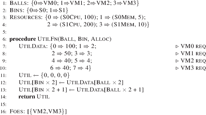
We begin by mapping our problem onto balls, bins, resource dimensions, and capacity constraints (Specification 1, lines 1–4). The Balls list comprises the VMs, and the Bins list contains the servers. Resources defines 4 dimensions: the first two capture the CPU and memory of server S0. The next two capture the CPU and memory on server S1. Each dimension is specified with the corresponding capacity value.
Next, we capture requirement 1 of this example by defining a suitable resource utilization function. Lines 7–10 capture the resource utilization data in the UtilData array. The first two elements list VM0’s CPU and memory requirements respectively (line 7). The next two elements list VM1’s requirements, and so on. Note that UtilData exists only within the user-defined function, and is not part of the abstraction.
Line 11 initializes the utilization vector, which has the same number of elements as Resources. Lines 12 and 13 read the CPU and memory requirement of the given Ball from UtilData, and store them in the CPU and memory dimension for the given Bin in the vector.
Now, we capture requirement 2. Since VM2 and VM3 need to run on different servers, we define a foe set containing them (line 16). This completes the specification of the problem using Wrasse’s abstraction. A satisfying solution for this problem is to place VM0, VM1, and VM2 on S1 and VM3 on S0.
Wrasse uses massive parallelism by orchestrating hundreds to thousands of light-weight GPU threads to explore the search space in parallel. Our goals in designing the solver were:
Generic search: A key challenge in designing the Wrasse solver was to avoid the use of any tuning knobs, parameters, or magic numbers that may make it less generic.
Speed: At the same time, by exploiting design features of our language, Wrasse should find solutions quickly, taking at most a few seconds. One may ask if this is fast enough. Previous analysis (though unconfirmed) has conjectured that Amazon Web Services place roughly 50,000 instances per day [4] on their infrastructure. Assuming the number has since doubled, this amounts to placing roughly 1.15 instances per second. It turns out that we can achieve such speeds using Wrasse with only one GPU, and can enhance it further using a cluster of GPUs.
At a high-level the solver operates as follows: for each bin it considers all unallocated balls (in parallel). It invokes the user-defined utilization function with the partial assignment; checks that capacity constraints are met; assigns friend balls (if any) by repeating the same steps; and checks to ensure that no foe group is fully assigned to the same bin. If any constraint is violated, the ball is left as unallocated. When no more balls can fit, the solver moves on to the next bin, until all balls are allocated, or all bins are exhausted. The following sections describe various design decisions and implementation details of the Wrasse solver.
Exploiting Language Features. Consider our balls and bins abstraction — a ball can be put in only one bin. Our Wrasse solver has a straight-forward implementation: one integer variable for each ball (bi). This variable is set to a value that represents its bin (j). A generic constraint solver does not have the concept of balls and bins. We have implemented Wrasse’s abstractions on two different solvers (Z3 and ECLiPSe) and found that to get the best performance from these solvers, we needed to encode the constraints using a boolean variable for each ball-bin combination (bij). We ensure a ball can be put in only one bin through an additional constraint of the form ∃j′ ∀j ≠ j′ ¬ bij, which implicitly encodes a quadratic loop. Cologne [19] uses a similar formulation with the Gecode solver. Thus where generic constraint solvers require a quadratic number of variables and a constraint involving both an existential and a nested universal quantifier to encode the simple balls and bins abstraction, the Wrasse solver requires only a linear number of variables and no additional constraints.
For resource constraints, Wrasse maintains a single variable (per dimension) for the current resource utilization. When attempting to allocate a ball to a bin, Wrasse checks the variables corresponding to the dimensions affected (and updates them with the ball’s incremental contribution). In a generic constraint solver, the capacity constraint is specified as ∑i bij rid ≤ cjd where rid and cjd are ball i’s utilization and bin j’s capacity along dimension d respectively. Depending on the implementation, every time a generic constraint solver attempts to allocate a ball to a bin it must, for each dimension affected, either evaluate this constraint (linear in the number of balls), or devote quadratic storage (number of balls times bins) if it caches sub-terms and uses them for incremental updates. Our Wrasse solver achieves this incremental update with a constant storage and constant computational cost per dimension affected.
Similar gains are to be had for the friends-and-foes mechanism, and soft-constraints. The Wrasse solver is orders of magnitude faster than generic constraint solvers because it exploits our language features.
GPU. GPUs expose a large number of hardware threads, but each thread is less capable than a conventional CPU thread. Specifically, on-chip memory is highly constrained (few kilobytes), groups of threads (thread-groups) share a single instruction pointer (stalling as needed for correctness), and inter-thread communication is limited to (slow) memory barriers. To make best use of hardware, our implementation abides by three rules: 1) threads should ideally execute the same code-path (on different data), 2) they should collaborate to increase sharing of the limited on-chip memory, yet 3) avoid expensive synchronization and data-dependence across threads. Our language design was heavily influenced by these constraints.
One example is our design of the interface for the user-provided utilization function where we explicitly pass in the (read-only) partial allocation. Each thread in a thread-group allocates a randomly-selected ball to a bin. The problem is in picking the partial allocation for each thread. Note that if two threads are assigning two different balls to the same bin simultaneously, one thread cannot delay its execution until the other is done to accurately reflect some serialized order (violates Rule 3, no cross-thread data-dependence). Letting both allocate in parallel based on the current allocation is wasteful since even if they individually succeed in allocating their respective balls, it may not be possible to allocate both balls on this bin. To get around this problem, we pass different partial allocations to each thread. To the first thread we pass the current allocation, but to the second thread we pass a speculative allocation where we assume the first thread’s allocation succeeded. To the third thread we speculate that both the first two threads succeeded. We execute a single memory-barrier after the actual allocation result is available. Based on the actual results, we identify threads where we speculated correctly and reconcile their outputs.
Other GPU-specific optimizations which we leveraged include caching the problem specification and data in special off-chip GPU memory that is highly optimized for read-only access. This requires our specification language to be concise, as reflected in high-level abstractions like balls and bins rather than generic variables and equations.
Picking balls and bins. An interesting design question arises in how balls and bins are picked. Different choices optimize for different outcomes.
To optimize for an allocation that uses the fewest number of bins, we mentioned we pick one bin and attempt to assign each ball to that bin. Once the bin is full, we move on to the next bin. Thus each bin is packed to capacity and, although we do not guarantee it, in practice comes quite close to the optimal (see Section 8).
To optimize for an allocation that balances utilization across a fixed set of bins, each thread-group allocates balls to a set of bins, or a bin-group. Parallel threads attempt to assign each ball to a random bin in that group, resulting in a more even distribution.
An interesting design point is considering power-of-two sized bin-groups. This can exploit real-world spatial coherence in bins (if any exists) while being domain agnostic. Consider, for instance, servers (bins) connected to a tree-like network topology. Communicating VMs (balls) placed in the same sub-tree result in lower resource utilization (i.e., easier to find a satisfiable solution) than when placed in different sub-trees since in the latter scenario traffic needs to be routed through links outside the sub-trees. Power-of-two bin-groups effectively allow us to pack sub-trees before moving on to the next sub-tree.
Instead of requiring the user to specify the bin-group size, the Wrasse solver tries several in parallel. We devote some GPU thread-groups to size one, some GPU thread-groups to the maximum number of bins, and one each to size two, four, eight and so on. Our GPU supports running thirteen thread-groups in parallel. Thus we maximize our chances of finding a satisfiable solution without burdening the user with additional tuning knobs.
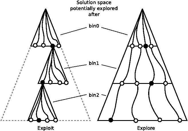
Explore vs. Exploit. The next interesting design point is balancing exploration vs. exploitation when moving on to the next bin-group. By exploitation we mean identifying one or more “good” partial solutions and promoting them to other thread-groups so multiple groups can build upon the good assignment(s). By exploration we mean each thread-group independently exploring its own partial solution as deep as possible. Figure 1 illustrates this choice. Both cases initially execute four thread-groups using a bin-group size of one, resulting in four different sets of balls being assigned to bin 0. In the exploit scenario, the best of the four partial solutions is picked, and the four threads assign balls to bin 1; all four have the same assignment for bin 0 but different assignments for bin 1. Again the best solution moves forward and balls are assigned to bin 2, and so on. Thus at step k, the assignment for bins 0…k−1 is the same and the threads randomly assign to bin k. In the explore scenario, each thread autonomously assigns balls to each bin in succession, and the solution after k steps is completely different for each bin.
We chose to explore rather than exploit in the Wrasse solver. This is primarily because defining the notion of a “good” partial solution in a domain-agnostic manner is problematic. Even if we were to ask the user for a heuristic (we do not), we found that in practice writing such heuristics is hard. In many cases we found the best solution (at the end of tens of steps) was because of a random lucky assignment in the very early steps. Writing a heuristic that has a lookahead of tens of steps is nearly infeasible. Exploration has three advantages: 1) we retain early lucky decisions, 2) after k steps we end up with a larger diversity of assignments (making it more likely that one of them is a near-solution), and most importantly, 3) we do not need heuristics.
The GPU threads exit after exhaustively attempting to assign balls to bins. If any of the thread-groups manages to finish assigning all balls, a solution has been found; the solver returns the assignment to the user and terminates. Otherwise our Wrasse solver terminates on user-interrupt or after a user-specified time interval (typically a minute or two).
The Wrasse service has a number of limitations, some fundamental, and some implementation-defined. In this section we discuss the key fundamental limitations of the Wrasse abstraction. We discuss limitations of our implementation in Section 7.
Cannot determine non-existence. The Wrasse service cannot determine when a solution does not exist. The solution search space is simply too large to explore in any reasonable time despite parallelism. Even when the problem size is extremely small, the use of randomness in exploring solutions (which is indispensable for large search spaces) means the service cannot guarantee exhaustive search for small search spaces. Overall, Wrasse is sound (i.e., any solution it finds is a valid solution), but not complete (i.e., it may not find a solution in reasonable time even if one exists).
Minimization. The Wrasse service does not guarantee a “minimal” solution; it merely returns a solution that satisfies the constraints. However, we can iteratively tighten the constraints to get close to the minimal solution. For example, the user cannot ask the service for the minimum number of bins that will fit the given balls. However, the service can run the same problem iteratively while reducing the number of bins until no solution is found in reasonable time, thereby finding a close-to-minimal solution.
Non-trivial transformations. The decision bin-packing problem, which is the abstraction offered by Wrasse, is NP-complete [9]. Thus, at least in theory, Wrasse is feature-complete, and any other problem in NP can be transformed into it. This includes all resource allocation problems that we have encountered in the cloud computing space. In practice, however, doing so efficiently can be quite non-trivial. The transformation complexity shows up in the imperatively-defined utilization function. One example is the job-scheduling problem discussed in Section 6.3. Efficiently encoding it requires two types of balls (a notion Wrasse doesn’t natively support). For problems that are a closer fit to bin-packing, however, the utilization function tends to be much simpler.
In this section, we show that Wrasse is general and extensible by specifying various extensions to the simple VM placement problem described in Section 3.4. We first concentrate on extending the VM placement specification to include time-varying requirements. We next show how Wrasse can capture network bandwidth constraints, which is an example of a shared resource. Finally, extend our specification to perform simultaneous scheduling of multiple jobs.
The Microsoft Assessment and Planning Tool (MAP) [20] uses a VM placement algorithm to help businesses determine how much it would cost to run their applications on an Azure [2] instance. MAP takes as input VM requirements as a function of time, i.e., for different time slots during the day (say per-hour), to capture the non-stationary behavior of certain VCs. For example, user-facing VMs may require more resources in the day than at night, while batch-processing VMs may do more work at night. Using non-stationary input allows for better VM placement since VMs with temporally anti-correlated resource utilizations can be placed on the same server, which we could not otherwise do taking only peak utilization into account.
To capture this scenario, for each original resource (e.g., S0Cpu in Specification 1) we create one resource dimension per time-slot (i.e., S0CpuT0, S0CpuT1, S0CpuT2, … each with the same capacity as for S0Cpu originally). Similarly, the scalar resource utilization in UtilData (line 1.7) is replaced with the time-varying utilization (e.g. 100 is changed to [20, 30, 100, …] corresponding to each time-slot) and the utilization function is changed to add the resource utilization corresponding to each resource and time-slot to the appropriate resource dimension. Temporally anti-correlated VMs will sum to lower combined utilization (along each individual time-slot dimension) than they would have if peak utilization was used; as long as the lower combined utilization does not exceed the capacity along any dimension, Wrasse may then assign them to the same bin.
A further relaxation commonly requested in real-world settings is the
95% rule, where server utilization may temporarily (say, for
only 5% of time-slots) exceed capacity by at most 10%. Using the soft
constraints mechanism in Section 3.3, the
user can add the line:
[{S0CpuT0, S0CpuT1, …}p=0.95, o=10%;…
Wrasse will then effectively allow assignments where a particular resource capacity is exceeded in only 5% of time-slots by requiring that p=95% of the time-slot dimensions for each group specified meet their capacity constraint (and the rest don’t exceed by more than o=10%).
The network virtualization problem as addressed by SecondNet [13] and Oktopus [6] extends the simple VM placement problem expressed in Section 3.4 with network bandwidth requirements. The two systems have very different abstractions and placement heuristics. Wrasse can model both.
SecondNet uses the abstraction of a virtual data center (VDC) for tenants to specify their requirements. Along with CPU, memory and disk requirements of VMs in a VDC, the specification includes pair-wise bandwidth requirements to one or more other VMs. Network links have associated bandwidth capacities. The added constraint is that communicating VMs be placed on servers so that they do not exceed the capacities of network links connecting those servers.
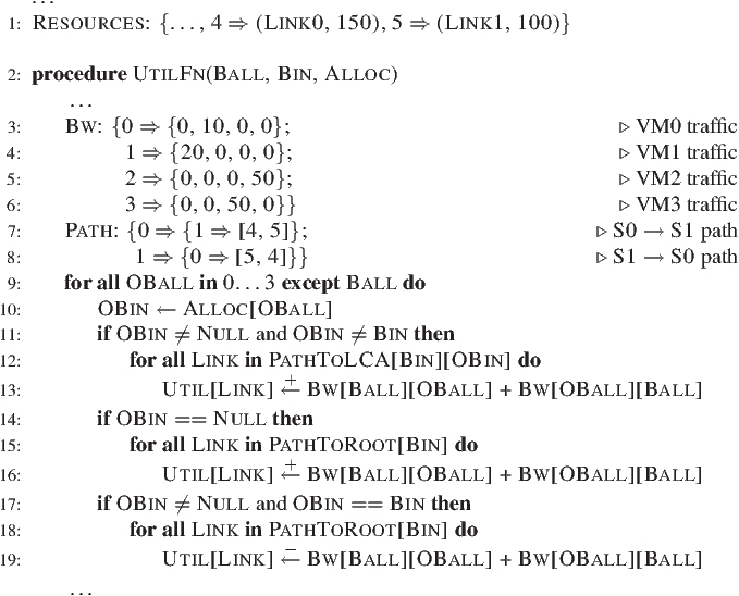
We extend the VM placement problem formulation in Section 3.4 to include the network bandwidth requirement as follows (all additions are shown in Specification 2). Each network link in the data center is represented as a resource dimension with the link capacity as the resource capacity. Say, in our example in Section 3.4, the two servers are in the same rack connected through a TOR switch. Therefore there are two network links between the servers. We augment the Resources vector in Specification 1 with these two network links and their capacities as shown in Line 1 of Specification 2.
We capture the pair-wise bandwidth in the resource utilization function as follows.
Step 1: We store the traffic matrix and routing information as data within the UtilFn (lines 2.3–2.8 in Specification 2). The Path value [4,5] (in line 2.7) is the route to get from server S0 to server S1: 4 and 5 are resource dimensions for Link0 and Link1 respectively2. As with UtilData, Bw and Path data is opaque to Wrasse.
Step 2: When a VM is to be placed on a server, then for every other VM that has already been placed on a different server (line 2.11), add the bandwidth requirement between this VM and the other VM on the path only up to the lowest common ancestor (half the path) of the VMs (lines 2.12, 2.13). We allocate bandwidth only on this VM’s half of the path because the other VM has already allocated bandwidth on its side as explained below.
Step 3: For every other VM that has not been placed (line 2.14), add the bandwidth requirement between this VM and the other VM on the path from this server to the root of the tree (line 2.15, 2.16). We make this addition to provision for the worst-case that all unallocated VMs might be placed on servers farthest from the current VM’s server, and thus all communication from this VM to the unallocated VMs may go up to the root of the tree.
Step 4: For every VM that is placed on the same server (line 2.17), subtract the bandwidth between the VMs (by stating a negative allocation) for all links from this server to the root (line 2.18, 2.19). This is because when the other VM was placed, it had provisioned for the worst-case and added the bandwidth requirement to links from this server to the root. Since both VMs ended up on the same server, we can take back this allocation. We repeat this subtraction for every pair of VMs that has a lowest common ancestor that is lower than the root (and is therefore not the worst-case), but leave out the pseudocode for simplicity.
As before, Wrasse proceeds with the assignment only if the added resource utilization returned by the UtilFn to the existing partial assignment does not exceed capacity constraints along any dimension, which in this case translates to respecting network link capacities for pair-wise bandwidth requirements. We have used this implementation of the SecondNet abstraction in our comparison in Section 8.2.1.
We briefly describe how we specify the Oktopus virtual network abstraction in Wrasse. The Oktopus Virtual Cluster (VC) abstraction specifies a virtual star topology with N VMs: a single virtual switch connects all VMs. Associated with each virtual link in the topology is a bandwidth requirement B. When this VC is placed on the network, on any physical link that VMs for this VC span, the VC requires a capacity reservation of min(m, N−m)*B, where a total of m VMs are placed on the sub-tree connected to the said link.3
The authors also describe a Virtual Oversubscribed Cluster abstraction that uses a two-level virtual tree topology. We can specify both abstractions using Wrasse though for brevity and ease of explanation, we concentrate on the VC abstraction.
As with Secondnet, each network link in the data center is represented as a resource dimension with the link capacity as the resource capacity. Assume the simplest network topology for this example as well – two servers linked through one switch. Therefore there are two network links between the servers. We proceed as follows:
Step 1: We store the number of VMs N in the VC and the bandwidth value B within the UtilFn. The paths between every pair of servers can be computed and stored in UtilFn.
Step 2: Say k VMs of this VC are already placed on a server. When a new VM VM1 is to be placed on this server, Then the number of VMs potentially placed outside this server is N−k−1 (including unallocated VMs). Using the minimum bandwidth calculation of Oktopus, we say that if (k+1 < N−k−1), the bandwidth usage on the link is (k+1)× B. else the bandwidth usage on the link is N−(k+1)× B. We write the Wrasse specification with the appropriate increments in bandwidth allocation to reflect this logic. Interestingly, this single step completely captures the Oktopus VC abstraction.
Section 8.2.2 evaluates our Oktopus implementation.
More complex topologies: We capture more complex network topologies such as Fat Trees and VL2 with appropriate additions to the Path data structure and the UtilFn logic. In a Fat Tree, there are multiple paths between any two servers in the data center network, and therefore a flow between two VMs on these servers can take any one of these paths. We briefly explain one way to capture this, though by no means is it the only way. When a VM is to be placed on a server, then for every other VM that has already been placed on a different server, add the bandwidth requirement from this VM to the other VM, divided by the number of forward paths between the servers, on all the forward paths from this server to the other VM’s server.
Adding path length constraints: In addition to bandwidth constraints, we can also extend the network virtualization specification to enforce a maximum path length constraint as in Rhizoma [28] between any two VMs.
In certain cloud-computing scenarios [6], there is some flexibility in scheduling multiple VCs simultaneously to better manage resources. We now introduce a notion of a tenant job (similar to a VC), which consists of a set of VM requirements that enters the system at a particular time, waits until resources are available, runs for some duration, and exits the system. We now have definitions of a batch of jobs simultaneously, and want to schedule both the job start time, and assign the job VMs to servers while satisfying capacity constraints.
Logically, we now need to have two types of balls — one type for jobs (J), and one type for VMs (V). We also need two types of bins — one type for job start time-slots (T), and one type for servers (S). Once Wrasse assigns a job to a start time-slot, the job runs for the number of contiguous time-slots specified in the job request. We define a resource dimension for each time-slot for each server resource (CPU, memory, etc.) as in Section 6.1. We could similarly define a resource dimension for each time-slot for each network-link, but we omit bandwidth requirements for brevity. We also define a dimension for total CPU (and memory) for each time-slot with the capacity set to the aggregate CPU capacity (and aggregate memory capacity) across all servers.
Job balls can only be placed in time-slot bins, and VM balls can only be placed in server bins, however, Wrasse does not differentiate between different types of balls. Nevertheless, we can enforce different ball and bin types using the existing Wrasse abstraction. We do this by adding a conflict dimension C with capacity 1, which is just like any other resource dimension. If there is a mismatch in the type of ball and bin (i.e., the solver randomly picks a job ball for server bin, or a VM ball for time-slot bin), the resource utilization function sets the conflict dimension utilization to 2, which clearly exceeds the capacity of C, resulting in the solver aborting that assignment and moving on to a different ball.
When placing job ball Ji into time-slot bin Tx, the resource utilization function computes the aggregate CPU and memory requirements for the job and increments the dimensions corresponding to the total CPU and memory resource for that time-slot, and k subsequent time-slots where k is the duration of the job. Thus if job Ji lasts 2 time-slots, resource dimensions ToalCpuTx, ToalCpuTx+1 and ToalMemTx, ToalMemTx+1 are incremented. This weeds out assignments of jobs to time-slots that would be impossible to satisfy, thereby reducing the search space for assigning VMs to servers. When placing a VM ball VMp into server Sm, the resource utilization function first checks the current partial assignment for the job Ji this VM is associated with. If that job has not been assigned, the function aborts the assignment by setting the conflict dimension utilization to 2. If that job has been assigned to time-slot bin Tx, say, the utilization function increments the resource dimensions corresponding to server and time-slot(s).
The above specification encodes a joint resource allocation problem into the existing Wrasse abstraction, which the Wrasse service finds a simultaneously satisfying assignment for.
We use a combination foe groups to capture the second requirement.
Hadoop’s rack-aware replica placement [14] places three data replicas: two on separate servers on the same rack, and one on a server on a different rack. We require two ball types and two bin types to represent this. We represent each replica with two balls: one that places on a “rack" bin (we call this a rack ball), and one that is allocated to a “server" bin (server ball). There are a total of 6 balls per data item.
To enforce placement objectives of replicas to racks, we use the “friend" and “foe" abstractions: rack-balls 1 and 2 are friends, rack-balls 1 and 3 are foes. This mapping captures replica-to-rack requirements. To place same-rack replicas on different servers, we state that server-ball 1 and server-ball 2 are foes. We order the placement of rack-balls first, and then the server-balls using the same techniques as with job scheduling.
CDN data Placement: We are working with the CDN administrators of a cloud computing provider to build a data placement engine using Wrasse. The requirements of the CDN are currently threefold. First, place data such that the network load is evenly split across all servers in the CDN PoP. Second, place replicas of data such that they are evenly split across machines served by two different sources of power, such that if one source of power fails, half the replicas will still be available. Third, each server has a restriction on the number of SSL-encrypted data-items it can serve.
We have encoded the first and the third constraints using the utilization function. To ensure that network load is evenly split across all servers, we configure the solver to run with a step size equal to the number of servers (bins), as explained in Section 4. We use the “foe" abstraction to catpure the second constraint.
Spain [22] requires a mapping of network paths to a minimal number of VLAN IDs as part of its multi-path routing protocol, subject to the constraint that the network paths assigned to a VLAN ID should not create a loop. We have used Wrasse’s abstractions to model this as well. Several other problems are amenable to being expressed in Wrasse’s abstractions, such as multicast in wireless networks in the DirCast system [8], VLAN assignments in enterprise networks [26], and server selection in wide-area content distribution networks [24].
We have built Wrasse as a web service. The front-end simply accepts requests in the Wrasse specification language. At the back-end, worker tasks running on commodity workstation hardware equipped with either ATI/AMD or Nvidia GPUs process submitted jobs and upload the result back. We have evaluated Wrasse on three different GPUs – a common desktop Nvidia Quadro, the AMD Radeon 6990: a high-end gaming GPU, and the Nvidia Tesla C2075: a GPU specifically designed for high-performance computing. We chose the Tesla for our evaluations since it provided the best memory performance.
Problem Wrasse LoC Heuristic LoC VM Placement 5 80 (FFDProd) SecondNet 48 1396 Oktopus 24 613 SecondNet+Job Scheduling 103 - Table 2: Wrasse specification size for different applications.
Application VMs Avg. CPU Avg. Memory Avg. Disk Av. Network out Avg. Network in (Fraction of Total CPU) (GB) (MBps) (MBps) (MBps) PgRank 474 0.16 2.94 7.67 1.95 2.03 ClkBot 885 0.14 1.07 19.69 0.78 1.22 ImgProc 2942 0.37 0.35 1.41 0.92 0.04 Table 3: Resource requirements of applications.
Wrasse is written in a combination of C (for the CPU parts), and OpenCL (for the GPU parts). It consists of 1079 source lines of code including 347 lines for parsing the input specification, and 453 lines that run inside the GPU. In addition, table 2 shows the lines of code of the utilization function for different problem specifications. The number of lines is typically very small, ranging from 5 lines for the simple VM placement problem, to 103 lines to encode VM placement with SecondNet’s network virtualization abstraction and job scheduling. We have encoded SecondNet assuming a Fat Tree topology, and Oktopus using a simple tree topology.
We have obtained the implementations of the heuristics from the authors of SecondNet and Oktopus for comparison. The SecondNet heuristic consists of 1396 lines of C++ code, and Oktopus has 613 lines of C# code. The corresponding lines of code in Wrasse are 48 and 24. We have also encoded various well-known VM placement heuristics for comparison: the FFDProd heuristic [18] uses 80 lines of code.
Limitations. Our Wrasse solver accepts arbitrary OpenCL code in the user-defined utilization function. Since this function is called many times, the performance of our solver depends, in part, on the performance of this code. Thus user code that is inefficient or makes suboptimal use of the GPU memory hierarchy will directly impact performance. Given the memory budget, one approach we found useful (and performant) was to trade off data storage for computation. For example, instead of passing pre-computed Fat Tree routes, we compute the route in the utilization function saving several kBs of memory.
In this section, first, we compare Wrasse’s specification of VM placement with that of well-known heuristics as well as a generic constraint solver-based approach. We evaluate the simplest specification first to show the basic benefits of using Wrasse. Next, we present a comparison of Wrasse’s solution quality and performance for the network virtualization problem using both SecondNet and Oktopus. Finally, we investigate the benefits of using a GPU-based solver over a traditional CPU-based approach.
We use the VM placement specification from Section 3.4 to compare Wrasse’s solution quality and performance with state-of-the-art heuristics, and a specification of the same problem using the Z3 constraint solver [10]. The objective of this experiment was to determine whether Wrasse provides solutions as good as heuristics designed carefully and specifically for the VM placement problem, and to determine how Wrasse’s performance compares with those of the heuristics, and the generic constraint solver.
All experiments were run on a machine with an Intel processor running at 3.0GHz with 4GB memory. Wrasse used the same setup with an Nvidia Tesla C2075 GPU which can run 2048 threads in parallel configured into 256 groups.We used Nvidia’s GPU computing SDK in all our experiments.
We ran three heuristics [18] that are used by Microsoft’s System Center Virtual Machine Manager: FFDProd, Dot-Product, and Norm-based Greedy (NBG). Each heuristic takes five resource requirements from each VM – CPU, memory, disk, outbound network bandwidth, and inbound network bandwidth. The FFDProd heuristic is based on the first-fit decreasing paradigm [9]. It combines all five dimensions into one scalar quantity, calculates a similar scalar quantity for each server, and place VMs on servers based on a function of the two scalar quantities. Dot-Product and Norm-based Greedy (NBG) are dimension-aware heuristics that use multi-dimensional vectors to do the placement. Note that the network bandwidth resource here is used purely to determine if the server’s NIC is capable of providing that bandwidth. It does not involve the data center network in any way.
We used the Z3 Satisfiability-Modulo-Theory (SMT) solver to evaluate the constraint-solver based approach. The input to Z3 were a set of five constraints - one for each dimension – stating that the total resources used on each server should be less than the capacity of the server. Also, we input the maximum number of servers available for the placement.
The servers in the data center are considered homogeneous with 8 CPU cores, 16GB memory, 128MBps network bandwidth, and 50MBps disk bandwidth. Our evaluation used data collected from three cluster-based applications as shown in Table 3: a pagerank algorithm (PgRank), a machine-learning based click-bot detection algorithm (ClkBot), and a parallel image processing algorithm (ImgProc). For each dataset, we ran every experiment 5 times and present the average of the runs in the results.
Z3 did not scale with any of the three datasets, running beyond 12 hours with each dataset. Therefore, when running with Z3, we partitioned each dataset into smaller sub-problems – 5 for PgRank, 9 for ClkBot, and 30 for ImgProc – and ran the partitions in parallel.
Application FFDProd DotProd NBG Z3 Wrasse PgRank 90 100 97 90 89 ClkBot 420 420 420 424 420 ImgProc 1406 1403 1406 1417 1403 Table 4: Solution quality, comparing three production-level heuristics, the Z3 solver, and Wrasse. Smaller is better.
Application FFDProd DotProd NBG Z3 Wrasse PgRank 7 16.2 19.2 30864 51 ClkBot 15.6 69.2 82.6 146149 7645 ImgProc 92.6 744.2 923.6 139876 370 Table 5: Runtime of heuristics, the Z3 solver, and Wrasse in ms.
Table 4 summarizes, for the three applications, the number of servers that each approach used to place the VMs. The fewer the number of servers used, the better since a tighter placement makes more economical use of the data center’s resources. With PgRank, Wrasse found a placement with 89 servers, whereas the best heuristic (FFDProd) found a solution only with 90 servers. We calculated the lower-bound for PgRank as explained in Section 3.3 as 88 servers. Therefore Wrasse found a solution within 1 bin of the lower bound. A savings of one server for one set of VMs may not account for much, but with thousands of tenants being housed in a single data center, even a saving of one server per placement can cause significant cost savings.
For both ClkBot and ImgProc, Wrasse found a solution that was as good as the best heuristic. Hence we find that Wrasse provides as good, if not better, solutions than the heuristics for all three applications. The constraint solver was unable to match up with either the heuristics or Wrasse. This is a consequence of partitioning the problem – smaller partitions appear to significantly curtail the search space for the solver to explore and find better solutions.
A conclusion we draw from this experiment is that, for the VM placement problem, in spite of using a more generic abstraction, Wrasse is able to match (if not improve) the performance of the carefully-tuned, production-level VM Placement heuristics. The explanation for this lies in the “explore” approach that Wrasse employs as explained in Section 4.2. Each GPU thread uses a completely different, randomized placement of balls to bins as it starts exploring the search space, thereby searching in parallel through different regions in the solution space. Each heuristic on the other hand uses a single (greedy) deterministic strategy to find a placement.
We now compare the performance of the heuristics, the constraint solver, and Wrasse. Table 5 summarizes the results. Wrasse takes 51 ms to find a solution for PgRank, and it took 7.6 seconds to produce the solution for ClkBot. On the other hand, all the heuristics take less than 20 ms to run. While Wrasse run-times can be much higher than that of heuristics, we believe that a run-time of a few seconds or less is acceptable for the problems that involve placement of VMs, since the algorithm is run the first time a request is scheduled onto the data center infrastructure. In spite of partitioning the problem, and providing worse solutions, Z3’s performance is roughly two orders of magnitude worse than that of Wrasse.
We now compare Wrasse’s specification of SecondNet and Oktopus with their respective heuristics. Broadly, both heuristics, proposed by the authors of the respective systems, find the smallest sub-tree in the network that can fit a Virtual Cluster, and then use different algorithms to allocate it within the sub-tree.
We have obtained code for both the heuristic placement and generating input from the authors of SecondNet to perform this comparison. We assume a data center network consisting of 1024 servers connected through a 2-level Fat Tree topology. Each switch in the tree has 16 ports. Each server has 16 cores (we assume we can place at most 1 VM on a core), 8G memory, and 1 Terabyte disk. Every link in the Fat Tree had 1 Gbps link capacity.
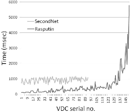
We generated two datasets for this evaluation. Dataset 1 (DS1) consists of a 300 VDCs each consisting of 100 VMs. Each VM used 256M memory, and 10 GB disk. Each VDC’s total bandwidth usage is randomly chosen to be between 50 and 150 Mbps, and this aggregate is used to generate the traffic matrix for each VDC randomly. Dataset 2 (DS2) also had 300 VDCs, but with VM numbers per VDC ranging from 64 to 128. All other parameters remain the same. Our choice of parameters was driven by the numbers quoted by the authors in the SecondNet paper.
Dataset SecondNet Heuristic Wrasse DS1(100 VMs per VDC) 94 150 DS1(64-128 VMs per VDC) 129 221 Table 6: Solution quality comparison between Wrasse and the SecondNet heuristic.
Solution quality: Table 6 summarizes our results for this comparison. For DS1, SecondNet placed 94 VDCs before hitting one that it could not place. On the same physical infrastructure and with identical input, Wrasse placed 150 VDCs before it could not allocate a VDC: a 56% increase. For DS2, SecondNet placed 129 before declining its first VDC, while Wrasse placed 221, an increase of 71%. We communicated our findings with SecondNet’s system designers to understand the large discrepancies. They informed us that their heuristic did not work well for VDCs larger than their “cluster size": a parameter that is hard-coded in the heuristic. This again reveals the benefit of a massive parallel search as opposed to parametrized heuristics.
Performance: We now analyze the run-time of the two approaches. The objective is not to compare the two run-times (we expect targeted heuristics to work much faster than Wrasse) but to show that Wrasse’s parallel search for allocations provides high-quality solutions within a few seconds at most, a goal we had aimed for.
SecondNet ran on a machine with a 3GHz Intel P2 processor with 4GB memory. Figure 2 shows the time to place each VDC for DS1. Interestingly, in the initial part of the placement, Wrasse performs better than the heuristic. Once finding solutions becomes difficult, the heuristic gives up, but Wrasse finds many more solutions albeit taking much longer – 5.8 seconds for the 150th VDC – to find a solution. Results are similar for DS2. On average, Wrasse took 525 ms to place a VDC, SecondNet took 925 ms.
Given that many data-center management allocation problems – almost all we have mentioned in this paper – do not require millisecond-level turnaround time on generating solutions, these run-times show that it is entirely feasible to use Wrasse to find high-quality allocations thereby leading to potential cost savings.
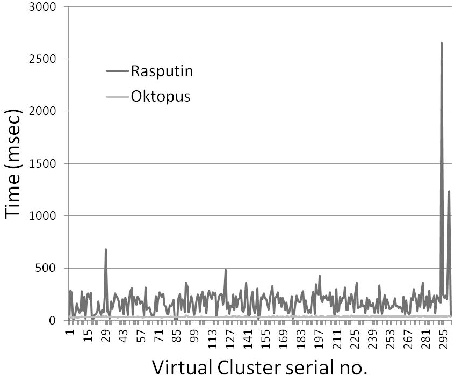
We have obtained code for the Oktopus heuristic from the authors for this comparison. In this experiment, the input to both Wrasse and the Oktopus heuristic consists of a set of 300 VCs, with VM numbers (N) ranging from 10 to 340. Bandwidth requirements (B) varied from 10 to 100 Mbps per VC.
The network we consider here is the same as in the Oktopus [6] evaluation: a 3-level tree topology with one aggregation switch connected to 10 pods, each pod connects to 40 TOR switches, and each TOR switch connects to 40 servers. Therefore the network has 16,000 servers, and 16,410 links. Each server can hold 4 VMs, and each network link has 1 Gbps capacity.
Both Wrasse and Oktopus placed all 300 VCs successfully. Figure 3 compares the placement time for each VC. Wrasse ran slower than the Oktopus heuristic here. Also, Wrasse took significantly longer (up to 2.6 seconds) to place certain VCs, the reason being that these VCs are particularly large in size with high bandwidth requirements, and the random search took that much time to find a feasible solution. The heuristic on the other hand has the benefit of knowing the smallest sub-tree in the network that fits this VC. The average time Wrasse took to place a VC for this dataset is 183 ms, whereas the Oktopus heuristic took 35.61 ms. Because of a (fixable) inefficiency in the utilization function, we could not run this experiment for larger sets of VCs. As we have mentioned, writing a good GPU-optimized utilization function is key to the implementation of Wrasse working well.
Finally, we evaluate the benefits and trade-offs of implementing the Wrasse service on a GPU-based architecture vs. a CPU-based architecture. For this purpose we implemented a multi-core optimized version of the Wrasse solver for CPUs. We ran the CPU-based version on a dual-core 3.0GHz Intel Core 2 Duo processor. We compare the throughput that the CPU and GPU implementations yielded.
We evaluated this with VM placement example using the PgRank data. Our GPU implementation on the Nvidia card has a throughput of 8127 solutions checked per second, while our CPU implementation checks only 966 solutions per second. This represents a 8.5x performance gain. We believe that by extending Wrasse to use a cluster of commodity GPUs, we will be able to drive these throughput numbers even higher.
We have presented Wrasse, a tool that provides a generic and extensible interface to solve resource allocation problems. At the front-end, the service supports a simple abstraction that we show is able to capture several data center resource allocation problems. At the back-end, Wrasse harnesses the power of GPUs to implement a massively parallel solver for the decision-version of the bin-packing problem. Our evaluation shows that Wrasse performs well, running to completion within a few seconds, while providing solutions that are as good as those provided by heuristics specifically designed for these problems.
This document was translated from LATEX by HEVEA.